Chapter 16 Monte Carlo
16.1 Introduction
The use of simulations can be useful and precise when obtaining explicit expressions is impossible or when numerical calculations are too time-consuming, as in the following example.
Example 16.1 In the case of the traveling salesman problem, the goal is to find the optimal route for visiting \(n\) cities in order to minimize the traveled distance. This involves calculating the length of \((n-1)!\) trajectories. With just 12 cities to visit, there are already 40 million trajectories to compute. However, simulation methods, based on iterative minimization (similar to genetic algorithms, where, starting from a route, two cities are randomly chosen and their positions in the current path are swapped), can approximate the optimum. While it may not guarantee the best solution (which is infeasible for \(n>20\)), it provides a very good solution with a high probability.
As we have seen in detail in Chapter 3, the central tool in non-life insurance is the pure premium, which is essentially a mathematical expectation (under the conditions of the law of large numbers). However, calculating the expectation of a random variable \(X\) with distribution function \(F\) often involves computing \(\int xdF(x)\). This calculation can be complex. A numerical method involves simulating \(X\) a “large” number of times, independently, and approximating the expectation as the empirical mean of the obtained realizations \(x_1, \ldots, x_n\), i.e., \[\begin{equation*} \frac{1}{n}(x_{1}+\ldots+x_{n}) \approx \mathbb{E}[X], \end{equation*}\] by virtue of the law of large numbers (Chapter 3, Property 3.5.2). It’s worth noting that we can also often assess the order of magnitude of the error. Indeed, if \(\mathbb{E}[X^{2}]<\infty\), then by the central limit theorem (Chapter 4, Theorem 4.2.1), when denoting the error as \(\varepsilon _{n}=(X_{1}+\ldots+X_{n})/n-\mathbb{E}[X]=\overline{X}-\mathbb{E}[X]\), we have \[\begin{equation*} \sqrt{n}\frac{\varepsilon _{n}}{\sqrt{\mathbb{E}[X^{2}]-\left(\mathbb{E}[X]\right)^{2}}}\rightarrow_{\text{distribution}}\mathcal{N}or\left( 0,1\right) . \end{equation*}\] In practice, this yields a 95% confidence interval for the expectation, approximated by \[\begin{equation*} \left[ \overline{x}-1.96\frac{s _{n}}{\sqrt{n}},\overline{x}+1.96\frac{s _{n}}{\sqrt{n}}\right], \end{equation*}\] where \(s _{n}^{2}\) unbiasedly estimates the variance of \(X\), i.e., \[\begin{equation*} s _{n}^{2}=\frac{1}{n-1}\sum_{i=1}^{n}\left( x_{i}-\overline{x}\right) ^{2}. \end{equation*}\] This allows us to determine the number \(n\) of simulations required to achieve the desired level of precision.
In general, Monte Carlo methods have been widely used to approximate integrals of the form \(\int_{0}^{1}g\left( x\right) dx\). Notably, if \(U\sim\mathcal{U}ni(0,1)\), then \(\int_{0}^{1}g\left(x\right)dx=\mathbb{E}\left[ g\left(U\right)\right]\) can be approximated by \(\frac{1}{n}\left(g\left(u_{1}\right)+...+g\left( u_{n}\right) \right)\), where the \(u_{i}\) are random samples from $ni(0,1) $, demonstrating the close relationship between evaluating integrals through simulation and mathematical expectations. If the convergence rate is slower compared to standard numerical methods (on the order of \(\sigma/\sqrt{n}\)), it’s important to note that here, no regularity properties are assumed for \(g\) (unlike standard numerical methods). The convergence in $O(1/) $ is a drawback, but it can be shown that for multiple integrals, the speed remains the same (unlike standard numerical methods). Specifically, if \(U_1,U_2,\ldots,U_d\) are independent random variables with \(\mathcal{U}ni(0,1)\) distribution, then \[\begin{eqnarray*} \int_0^1\ldots\int_0^1g(x_{1},...,x_{d})dx_{1}...dx_{d} &=&\mathbb{E}[ g\left( U_{1},...,U_{d}\right) ] \\ &\approx &\frac{1}{n}\sum_{i=1}^{n}g\left( u_{i,1},u_{i,2},...,u_{i,d }\right) \end{eqnarray*}\]% still converges in \(O(1/\sqrt{n})\).
Example 16.2 This method can be used to approximate the value of $$. Indeed, it is easy to see that \[\begin{equation*} \pi =4\frac{\text{Area of the disk with diameter 2}}{\text{Area of the square with side length 2}}. \end{equation*}\]% Also, if $( X,Y) $ is uniformly distributed over the square $$, then we have \[\begin{equation*} \pi =\Pr\left[ X^{2}+Y^{2}\leq 1\right]. \end{equation*}\] This leads to the result presented in Figure ??, where we calculate the ratio of the number of realizations falling within the disk of radius 1 to the total number of simulations.
Remark. Note that Georges Louis Leclerc Buffon proposed a different method to calculate $$ in 1777, giving rise to the first historical example of using Monte Carlo methods. Consider a series of evenly spaced lines (strips of a smooth floor, a tiled floor, or a checkerboard) and a needle or a thin rod that is balanced such that its length matches the spacing between the lines. Toss the needle randomly onto the floor, recording \(X=1\) if the needle crosses a line and \(X=0\) otherwise. If this experiment is repeated \(n\) times, with \(p\) being the number of successes (\(X=1\)), then the proportion \(n/p\) should provide a good approximation of $$. For a 95% confidence interval, an accuracy of \(10^{-3}\) is achieved with 900,000 tosses.
FIG
The above illustrates the importance of generating random numbers from a \(\mathcal{U}ni(0,1)\) distribution. We will denote as a function that produces such random samples. Regarding the concept of randomness and random number generators on $$, it is essential to highlight the two most critical properties that a function must satisfy:
$( i) $ for any \(0\leq a\leq b\leq 1\),% \[ \Pr\Big[ \mathtt{Random}\in \left] a,b\right] \Big]=b-a\text{.} \]
$( ii) $ successive calls to this function must generate independent observations; that is, for any \(0\leq a\leq b\leq 1\), \(0\leq c\leq d\leq 1\)% \[ \Pr\Big[ \mathtt{Random}_{1}\in \left] a,b\right] ,\mathtt{Random}% _{2}\in \left] c,d\right] \Big] =\left( b-a\right) \left( d-c\right) \text{% .} \]% More generally, we refer to \(k\)-uniformity if, for any \(0\leq a_{i}\leq b_{i}\leq 1\), \(i=1,...,k\),% \[ \Pr\Big[ \mathtt{Random}_{1}\in \left] a_{1},b_{1}\right] ,...,% \mathtt{Random}_{k}\in \left] a_{k},b_{k}\right] \Big] =\prod_{i=1}^{k}\left( b_{i}-a_{i}\right) \text{.} \]
In fact, the most intuitive and crucial notion of randomness has no connection with the concepts of uniformity and independence: randomness is what is unpredictable.
16.2 General Principles
The standard library of any computer programming language contains a “random generator,” hereafter referred to as \(\mathtt{Random}\), which provides a sequence of numbers \(x_{1},...,x_{n}\) in \([0,1]\), indistinguishable from realizations \(X_{1}(\omega),...,X_{n}(\omega)\) of \(n\) independent random variables with the same \(\mathcal{U}ni(0,1)\) distribution. The randomness is revealed through successive calls to this function.
16.2.1 Pseudo-Random Numbers
There are many methods to simulate uniform distributions, known as random number generators or pseudo-random number generators. The general idea is to construct a random number generator by drawing uniformly from ${ 0,1,….,M-1} $, where \(M\) is a “large” number (on the order of \(10^{8}\)), and then dividing by \(M\) to obtain “real” numbers in $$.
To generate a sequence of pseudo-random numbers in ${ 0,1,….,M-1} $, starting with a seed \(u_{0}\), we construct a sequence $u_{n+1}=g( u_{n}) $ where \(g\) is a function defined on ${ 0,1,….,M-1} $ with values in ${ 0,1,….,M-1} $. The most commonly used method is the “congruential generators,” where the function \(g\) is of the form \[\begin{equation*} g\left( u\right) =\left( Au+B\right) \text{ modulo }M. \end{equation*}\]
The modulus \(M\) is often a power of 2 (\(2^{16}\) or \(2^{32}\)) because division by \(M\) is numerically easier. Another common choice is \(2^{32}-1\), which has the advantage of being a prime number. The period is the largest number of integers in \({0,...,M-1}\) that can be generated. Arithmetic conditions on \(A\), \(B\), and \(M\) are imposed to achieve the largest possible period.
Remark. The choice of constants \(A\), \(B\), and \(M\) is a fundamental issue in simulation. Figure ?? shows a three-dimensional plot of points $( U_{i+1},U_{i},U_{i-1}) $ - 3000 simulations - using the \(RANDU\) algorithm from IBM (\(A=65539\), \(B=0\), and \(M=2^{31}\)) and one of those proposed by (L’Ecuyer 1994) (\(A=41358\), \(B=0\), and \(M=2^{31}-1\)). Note that \(65539=2^{16}+3\), and it can be shown that for the \(RANDU\) algorithm, \[ U_{n+1}-6U_{n}+9U_{n-1}=0\text{ mod }1, \] which results in planes in the point cloud. This generator can pose serious problems due to the dependence that exists between the draws. In contrast, (L’Ecuyer 1994)’s algorithm does not reveal any structure in the generated triplets $( U_{i+1},U_{i},U_{i-1}) $.
FIG
In general, simulating random variables (of any kind) relies on simulating \(\mathcal{U}ni(0,1)\) variables. This will be the case, in particular, for the inversion method based on Proposition 2.5.2 from Volume 1. More generally, we can note the following result, which extends Proposition 2.5.2 to arbitrary dimensions.
Lemma 16.1 For any random vector \(\boldsymbol{X}\,\) in \({\mathbb{R}}^{d}\), there exists \(\Psi :% \R^{n}\rightarrow \R^{d}\) almost surely continuous such that $={}( U{1},…,U_{n}) $ where \(U_{1},...,U_{n}\) are independent and identically distributed as \(\mathcal{U}ni(0,1)\).
It is possible for \(n\) to be infinite here. Furthermore, the central assumption is that the \(U_{i}\) are independent (they can follow a distribution other than the uniform distribution).
Example 16.3 If $( u) =-( u) /$, then $( U)xp() $ when \(U\sim\mathcal{U}ni(0,1)\). This is a direct application of Proposition 2.5.2.
Example 16.4 If \[ \Psi \left( u_{1},u_{2}\right) =\sqrt{\left( -2\log u_{1}\right) }\cos \left( 2\pi u_{2}\right), \] then \(\Psi \left( U_{1},U_{2}\right) \sim\mathcal{N}or(0,1)\) when \(U_1\) and \(U_2\) are independent and identically distributed as \(\mathcal{U}ni(0,1)\).
Example 16.5 If $( u_{1},…,u_{n}) =_{i=1}^{n}[ u_{i}p] $, then \(\Psi \left( U_{1},...,U_{n}\right) \sim\mathcal{B}in(n,p)\) when \(U_1,\ldots,U_n\) are independent and identically distributed as \(\mathcal{U}ni(0,1)\)
16.2.2 The Inversion Method
16.2.2.1 The General Case
This method is the simplest of simulation methods and is based on the following property (Proposition 2.5.2 from Volume 1): let \(F\) be a distribution function defined on \({\mathbb{R}}\), and let $U( 0,1) $, then $X=F^{-1}( U) $ has the distribution function \(F\).
Example 16.6
If \(F\) is the distribution function corresponding to the \(\mathcal{E}xp(\lambda)\) distribution, then $F^{-1}(x)=-( 1-u) /$, leading to the simulation algorithm,Note that it is equivalent to consider $( ) $ and $( 1-) $, which follow the same distribution.
n <- 100000
u <- runif(n)
x <- -log(1-u)
16.2.2.1.1 The Discrete Case
This method can also be used for discrete distributions (including those taking values in \({\mathbb{N}}\)), especially if there exists a recurrence relation for calculating \(\Pr% [ X=k+1]\) from \(\Pr\left[ X=k\right] .\)
If we denote \(q_{k}=\Pr[X\leq k]\), then, with the convention \(q_{-1}=0\),%
\[\begin{equation*}
X=\min \left\{ k\in\mathbb{N}|q_{k-1}\leq U<q_{k}, \text{ where }U\sim
\mathcal{U}ni \left( 0,1\right) \right\} .
\end{equation*}\]%
Suppose there exists a recurrence relation between
\(\Pr[X=k+1]\) and \(\Pr[X=k]\), of the form
\[\begin{equation*}
\frac{\Pr[X=k+1]}{\Pr[ X=k] }=f\left(k+1\right) ,
\end{equation*}\]%
then the algorithm can be written as
Algorithm: My algo
- \(U\longleftarrow \mathtt{Random}\) and \(T\longleftarrow \mathtt{Random}\),
- \(a\longleftarrow 1-U\), $bT(a)^{2}-$, \(c\longleftarrow\left[\theta +1\right] -2\theta aT\) and $dc^{2}-4b(T-1) $,
- $V-/$.
il} \(U>q\) \end{quote} A very useful special case for actuaries is that of the Panjer family of distributions, as presented in Section 6.4.
16.2.3 Rejection Method
This method can be used if one wants to simulate a distribution, knowing that it is the conditional distribution of a distribution that can be simulated.
Example 16.7 Trivially, if \(0<\alpha <1\) and we want to simulate \(X\sim\mathcal{U}ni(0,\alpha)\), we can note that \(X\) has the same distribution as $[U|U] $ where $Uni( 0,1) $. It is sufficient to implement the following algorithm:
Algorithm: Rejection method
- Repeat \(X\longleftarrow \mathtt{Random}\),
- Until \(X\leq \alpha\)
Example 16.8 It is also possible to simulate a pair $(X,Y) $ uniformly distributed over the unit disk. For this, we simulate a pair $(X,Y) $, uniformly distributed over the unit square $$, until it falls within the unit disk:
Algorithm: Rejection method
- \(X\longleftarrow 2\times \texttt{Random}-1\)
- \(Y\longleftarrow 2\times \texttt{Random}-1\)
- Until \(X^{2}+Y^{2}\leq 1\)
However, Example 16.7 is not the optimal method for simulating a realization of the uniform distribution on $$, especially if $$ is small. Indeed, the number of iterations required follows a geometric distribution with parameter $$, whose expectation is $1/$. In Example 16.8, the average number of iterations is% \[\begin{equation*} n=\frac{\text{Area of the unit disk} }{\text{Area of the unit square}}=\frac{\pi }{4}\approx 1.27. \end{equation*}\]
n <- 100000
u <- runif(n, -1, +1)
v <- runif(n, -1, +1)
s <- sqrt(u^2+v^2)
mean(s<=1)*4
More generally, the following result is used, which allows simulating a random variable with any density \(f\) from an easy-to-simulate density \(g\).
Let \(f\) and \(g\) be two densities such that there exists a constant \(c\) such that $cg( x) f( x) $ for all \(x\). Let \(X\) be a random variable with density \(g\), and let \(U\sim\mathcal{U}ni(0,1)\), independent of \(X\). Then, the conditional distribution of \(X\) given \(U <h\left( X\right)\) has density \(f\), where \(h(x)=f(x)/cg(x)\). Also, if \(U_1,U_2,\ldots\) are independent and identically distributed with \(\mathcal{U}ni(0,1)\), and \(X_1,X_2,\ldots\) are independent and identically distributed with density \(g\), then by defining \[ \tau=\inf\{i\geq 1| U_i\leq h(X_i)\}, \] \(X_\tau\) will have density \(f\).
Proof. Let \(U\sim\mathcal{U}ni(0,1)\), and define \(h(x)=f(x)/cg(x)\). Then, if \(X\) has density \(g\), \[ \Pr[U>h(X)]=\int_{-\infty}^{+\infty} \int_{h(y)}^1 g(y)dudy=1-\frac{1}{c}. \] Furthermore, for \(t\in{\mathbb{R}}\), \[\begin{eqnarray*} \Pr[X_\tau\leq t]&=& \sum_{k=1}^{+\infty}\Pr[\tau=k,X_\tau\leq t]\\ &=&\sum_{k=1}^{+\infty}\Pr[U_i>h(X_i)\text{ for }i=1,\ldots,k-1]\Pr[U_k<h(X_k),X_k\leq t]\\ &=&\sum_{k=1}^{\infty}\left(1-\frac{1}{c}\right)^{k-1}\int_{-\infty}^t \int_{0}^{h(z)} g(z)dzdu\\ &=&\sum_{k=1}^{+\infty}\left(1-\frac{1}{c}\right)^{k-1}\int_{-\infty}^t g(z)h(z)dz=\int_{-\infty}^t f(z)dz, \end{eqnarray*}\] which means that \(X_\tau\) has density \(f\).
Note that the probability densities involved in the result can be either discrete or continuous. Counting distributions can also be simulated using this method. The rejection algorithm is then written as follows:
Algorithm: Rejection method
- Repeat \(X\longleftarrow \mathtt{simulate\ according\ to\ density\ }g\)
- \(U\longleftarrow \mathtt{Random}\)
- Until \(c\times U\leq f\left( X\right) /g\left( X\right)\)
Example 16.9
Consider the random variable \(Y\) with density \[\begin{equation} g\left( x\right) =\left\{ \begin{array}{l} 3\left( 1-x^{2}\right) /4,\text{ on }\left[ -1,1\right].\\ 0,\text{ otherwise.} \end{array} \right. (\#eq:DensFig15.3) \end{equation}\] It is then possible to use either of the two following methods to simulate such a distribution:Example 16.10 As we have seen in Example 16.3, it is straightforward to simulate an exponential distribution using the inversion of the cumulative distribution function. Noting that for all \(x\geq 0\), \[\begin{equation*} \frac{1}{\sqrt{2\pi }}\exp \left( -\frac{x^{2}}{2}\right) \leq \frac{\exp \left( 1/2\right) }{\sqrt{2\pi }}\exp \left( -x\right) , \end{equation*}\]% we can simulate a normal distribution using the rejection method from the simulation of the \(\mathcal{E}xp(1)\) distribution. If \(U\sim\mathcal{U}ni(0,1)\) and \(X\sim\mathcal{E}xp(1)\), the rejection inequality is then written as% \[\begin{equation*} \exp \left( 1/2\right) \exp \left( -X\right) U\leq \exp \left( -X^{2}/2\right) . \end{equation*}\]% This inequality can also be simplified by taking the logarithm: \(\left( 1-X\right) ^{2}\leq -2\log U.\)% Therefore, to simulate a variable with \(\mathcal{N}or(0,1)\) distribution, we simulate two independent random variables from \(\mathcal{E}xp(1)\), \(X\) and \(Y\), until \(\left( 1-X\right) ^{2}\leq 2Y\) since \(-\ln U\sim\mathcal{E}xp(1)\). We randomly select the sign \(S\) according to the \(\mathcal{B}er(1/2)\) distribution, and the product \(S\times X\) then follows the \(\mathcal{N}or(0,1)\) distribution. Figure ?? illustrates this procedure. We will see later that there are faster methods for simulating normal distributions.
FIG
16.2.4 Using Mixture Distributions
In the discrete case, suppose that the probability distribution of \(X\) can be written as% \[\begin{equation*} \Pr\left[ X=n\right] =\alpha p_{n}+\left( 1-\alpha \right) q_{n} \end{equation*}\]% where \(p_{n}=\Pr[Y=n]\) and $q_{n}=$, \(n=0,1,\ldots\) with \(0<\alpha<1\) Then, a simple way to simulate \(X\) is to simulate \(Y\) and \(Z\), and then set \(X=Y\) with probability $$ or \(X=Z\) with probability $1-\(. The algorithm is then written as follows: \begin{quote} \texttt{If }\)$ $% X$ $(p_{n}) $
$X$ $( q_{n}) $ \end{quote} In the continuous case, this method can also be used if the density of \(X\) can be written as a mixture.
16.3 Bootstrap Resampling
16.3.1 Principles
The bootstrap method is very practical (the term “to pull oneself up by one’s bootstrap” means “to get oneself out of a difficult situation” (from “The Adventures of Baron Munchausen”)). because it allows us to overcome sometimes restrictive assumptions about a family of probability distributions. In particular, this method is widely used to obtain better estimators from small samples (e.g., in actuarial reserving methods).
Let \(X\) be a random variable with cumulative distribution function \(F\), and assume that we have a sample \(X_{1},...,X_{n}\) following this distribution. We are then interested in studying the behavior of the function $T( X_{1},…,X_{n},F) $, which depends on the observations and the distribution function \(F\).
The bootstrap algorithm is as follows: 1. Starting from $% ={ X_{1},…,X_{n}} $, we calculate the empirical cumulative distribution function \(F_{n}\), defined as% \[\begin{equation*} F_{n}\left( x\right) =\frac{1}{n}\sum_{k=1}^{n}\mathbb{I}[X_{k}\leq x]. \end{equation*}\] 2. Conditionally on \(F_{n}\), we perform \(N\) equiprobable resampling with replacement in \(\mathcal{E}\): $% ^{}={ X_{1}{},…,X_{N}{}} $ is then the new sample ((Efron and Tibshirani 1994) suggested taking \(N=n\), however, better results can be obtained by sub-sampling and performing sampling without replacement (one can then reduce it to \(U\)-statistics)).We define the bootstrapped statistic $T^{}=T( X_{1}{},…,X_{N}{ },F_{n}) $.
We can then repeat the last step to obtain approximations using the Monte Carlo method. We repeat the second step $% m $ times, generating \(m\) samples \(% \mathcal{E}_{1}^{\ast },...,\mathcal{E}_{m}^{\ast }\), and observe \(m\) values \(T_{1}^{\ast },...,T_{m}^{\ast }\) of \(T\).
::: {.example} Let’s assume, for example, that $Xer(p) $, and let \(\widehat{p}_{n}\) be the frequency of \(1\) in the sample $={ X_{1},…,X_{n}} $, i.e., \(\widehat{p}_n=\frac{1}{n}\sum_{i=1}^nX_i\). Here, we consider \(T\left( \mathcal{E},F\right) =\widehat{p}_{n}-p\). The bootstrapped sample \(\mathcal{E}^{\ast }\) is then the sequence of \(N\) equiprobable resamples with replacement from \(\mathcal{E}\). Conditionally on \(\mathcal{E}\), the distribution of \(% X_{i}^{\ast }\) is therefore $er(_{n}) $% . The bootstrapped statistic \(T^{\ast }\) is% \[ T^{\ast }=T\left( \mathcal{E}^{\ast },F_{n}\right) =\frac{1}{N}% \sum_{i=1}^{N}X_{i}^{\ast }-\widehat{p}_{n}, \] for which we know the first two moments: \[ \mathbb{E}\left[ T^{\ast }\right] =0\text{ and }\mathbb{V}\left[ T^{\ast }\right] =% \frac{\widehat{p}_{n}\left( 1-\widehat{p}_{n}\right) }{N}\text{.} \]
xb <- sample(x, size = length(x), replace = TRUE)16.3.2 Bootstrap Confidence Intervals
Bootstrap can be useful when looking for a confidence interval for a parameter \(\theta\). In parametric statistics, \(\theta\) is generally estimated using maximum likelihood, which provides an estimator \(T\) and ensures the asymptotic normality of $T-$. Then, for a sufficiently large sample, we can deduce a confidence interval of the form% \[\begin{equation*} \left[ T-z_{1-\alpha }\sqrt{I^{-1}\left( T\right) },T+z_{1-\alpha }\sqrt{I^{-1}\left( T\right) }\right] . \end{equation*}\]% However, this result is only valid asymptotically and can be particularly poor in finite samples (especially if the sample is small) without normality assumptions. Without normality assumptions, it is necessary to estimate the quantiles \(T_{\alpha }\) and \(T_{1-\alpha }\) such that \(\Pr\left( \theta \in \left[ T_{\alpha },T_{1-\alpha }\right] \right) =\alpha .\)
Let \(G\) be the cumulative distribution function of $T-$, and \(G^{\ast }\) be the cumulative distribution function of \(T^{\ast }-T\), such that $T_{ }=G^{-1}( ) $ is estimated by $G^{}( ) $. In general, it suffices to use Monte Carlo methods, and we approximate \(G^{\ast }\) by% \[\begin{equation*} \widehat{G}^{\ast }\left( x\right) =\frac{1}{m}\sum_{i=1}^{m}\mathbb{I}% \left[ T_{i}^{\ast }-T\leq u\right] . \end{equation*}\]
Now, as we saw in Chapter 15, if \(X_{1},...,X_{n}\) are independent random variables with the same distribution function \(F_X\), an estimator of $F_X^{-1}( ) $ is \(X_{[\left( n+1\right) \alpha] :n}\). Therefore, \(T_{\alpha }\) can be approximated by \(\widehat{T}_{\alpha }=T_{\left( m+1\right) \alpha :m}^{\ast }\) (by choosing $$ and \(m\) such that $( m+1) $ and $( m+1) ( 1-) $ are integers; otherwise, interpolations can be used). Under these conditions, it is possible to show that \[ \Pr\Big[ \theta \in \left[ \widehat{T}_{\alpha },% \widehat{T}_{1-\alpha }\right] \Big] =\alpha +O\left( n^{-1/2}\right). \] One possible method to improve the convergence rate is to use studentized bootstrap (yielding an $O( n^{-1}) $ rate).
The use of bootstrap for heavy-tailed claims can pose several practical issues. Very large values tend to appear too frequently. As a result, bootstrap cannot be used to estimate an average or a probability of exceeding a value far from the mean.
Example 16.11 Figure ?? shows the estimation of the mean of \(n=100\) claims following $ar( 1,0) $ - on the left - and $ar( 2,0) $ - on the right. In the first case, the distribution does not have a finite mean, and in the second, the variance is not finite. The dashed curve represents the density of the normal distribution associated with the empirical mean and variance.
FIG
16.3.3 Bootstrap and Quantiles
As explained in detail in (Davison and Hinkley 1997), what legitimizes bootstrap is primarily the existence of an Edgeworth expansion for the statistic being calculated. Some statistics, especially empirical quantiles, can be irregular and unstable. While asymptotically these resampling methods are valid, the results at finite distances can be relatively poor.
16.3.5 Application to Loss Reserving
Consider the example of the log-Poisson regression (yielding the same estimators as the Chain Ladder method). For the data in Example ??, the graphical outputs of the regression are presented in Figure ??, including the deviance residuals and Pearson residuals. The Pearson residuals \(r_{i,j}^P\) are given in Table ??, and the deviance residuals \(r_{i,j}^D\) are given in Table ??.
FIG
Most stochastic models, as we have noted, have been implemented with the aim of replicating the Chain-Ladder method, to provide the same amount of reserves but allowing for error margin assessment. Using Monte Carlo methods, it is sufficient to independently simulate the increment errors, generate new triangles, and then use the Chain-Ladder method to obtain reserve amounts for this simulated triangle. If Pearson residuals are used, as recommended by (England and Verrall 1999), the bootstrapped increment is given by
\[ Y_{i,j}^* = r_{i,j}^{P*} \cdot \sqrt{\mu_{i,j}} + \mu_{i,j} \]
where \(r_{i,j}^{P*}\) is the bootstrapped Pearson residual.
16.3.7 Application to Loss Reserving
Let’s consider the example of the log-Poisson regression (providing the same estimators as the Chain Ladder method). For the data in Example ??, the graphical outputs of the regression are presented in Figure ??, including the deviance residuals and Pearson residuals. The Pearson residuals \(r_{i,j}^P\) are given in Table ??, and the deviance residuals \(r_{i,j}^D\) are given in Table ??.
FIG
Most stochastic models, as we have noted, have been implemented with the aim of replicating the Chain-Ladder method, providing the exact same amount of reserves while allowing for error margin assessment. Using Monte Carlo methods, it is sufficient to independently simulate the increment errors, generate new triangles, and then use the Chain-Ladder method to obtain reserve amounts for this simulated triangle. If Pearson residuals are used, as recommended by (England and Verrall 1999), the bootstrapped increment is given by
\[ Y_{i,j}^* = r_{i,j}^{P*} \cdot \sqrt{\mu_{i,j}}+\mu_{i,j} \]
where \(r_{i,j}^{P*}\) is the value of the bootstrapped Pearson residual.
In the case of the log-Poisson regression, the Pearson residuals are given in Table ??. A bootstrap simulation of the error yields the bootstrap residuals triangle in Table ??. If we return to the increments, defining \(Y_{i,j}^* = r_{i,j}^{P*}\sqrt{\mu_{i,j}}+\mu_{i,j}\), we obtain the values in Table ??.
Switching to the cumulative triangle, which can finally be completed using the standard Chain-Ladder method, we obtain the values in Table ??.
For this simulation, the required reserve amount amounts to \(425,160\). By repeating a large number of times (here \(50,000\)), we obtain the values in Table ??.
Remark. However, using the bootstrap on the triangle relies on very strong assumptions: the residuals must be independent and identically distributed. From a practical
16.4 Simulation of Univariate Common Probability Distributions
16.4.1 Uniform Distribution
We assume here that we have software capable of generating \(\mathcal{U}ni(0,1)\) random numbers, and we will refer to this function as .
n <- 100000
u <- runif(n, min=0, max=1)
16.4.2 Normal (Gaussian) Distribution
By applying the usual results on the normal distribution (see Section 2.5.4 of Volume 1), simulating a realization from the \(\mathcal{N}or(\mu, \sigma^2)\) distribution is straightforward. It involves generating a sample from the \(\mathcal{N}or(0,1)\) distribution and then properly transforming it (multiplication by \(\sigma\) and addition of \(\mu\)).
The following result provides an efficient method for simulating from the \(\mathcal{N}or(0,1)\) distribution.
Let $( X,Y) $ be a pair of random variables, uniformly distributed within the unit disk $={ ( x,y)2|x{2}+y^{2}} $. Denote \(R\) and $$ as the polar coordinates associated with $( X,Y) $, i.e., $X=R$ and $Y=R$. Let \(T=\sqrt{-4\log R}\), then $U=T$ and $V=T$ are independent and follow the \(\mathcal{N}or\left( 0,1\right)\) distribution.
Proof. Consider the change of variables that transforms Cartesian coordinates into polar coordinates, \[\begin{equation*} \phi :\left\{ \begin{array}{rcl} \mathcal{S}\backslash \left\{ \left] 0,1\right[ \times \left\{ 0\right\} \right\} & \rightarrow & \left] 0,1\right[ \times \left] 0,2\pi \right[ \\ \left( x,y\right) & \mapsto & \left( r,\theta \right)% \end{array}% \right. \text{ } \end{equation*}\]% and \[ \phi ^{-1}:\left\{ \begin{array}{rcl} \left] 0,1\right[ \times \left] 0,2\pi \right[ & \rightarrow & \mathcal{S}% \backslash \left\{ \left] 0,1\right[ \times \left\{ 0\right\} \right\} \\ \left( r,\theta \right) & \mapsto & \left( x,y\right) =\left( r\cos \theta ,r\sin \theta \right) ,% \end{array}% \right. \] with the Jacobian \(J_{\phi^{-1}}=r\). The density of the pair \(\left( R,\Theta \right)\) is then given by \[\begin{equation*} g\left( r,\theta \right) =\frac{r}{\pi }\mathbb{I}\left[ (r\cos \theta ,r\sin \theta )\in\mathcal{S}\right] , \end{equation*}\]% where the marginal distributions are respectively \[\begin{equation*} g\left( r\right) =2r\mathbb{I}\left[ 0<r<1\right] \text{ and } g\left( \theta \right) =\frac{1}{2\pi }\mathbb{I}\left[ 0<\theta<2\pi \right] . \end{equation*}\]% Hence, \(R\) and \(\Theta\) are independent, with \(R\) following a triangular distribution on \(\left] 0,1\right[\) and \(\Theta\) being uniformly distributed on \(\left] 0,2\pi \right[\). The distribution of \(T\) is then given by \[\begin{eqnarray*} \Pr[T\leq t] &=&\Pr\left[ \sqrt{-4\log R}\leq t\right]\\ &=&\Pr\left[ R>\exp \left( -\frac{t^{2}}{4}\right) \right]\\ &=&1-G\left( \exp \left( -\frac{r^{2}}{4}\right) \right) , \end{eqnarray*}\]% where \(G\) is the cumulative distribution function of \(R\). Thus, the density of \(T\) is \[\begin{equation*} t\mapsto t\exp \left( -\frac{t^{2}}{2}\right) \mathbb{I}\left[ t>0\right] . \end{equation*}\]% To determine the density of the pair \(\left( U,V\right)\), obtained by the change of variables \[\begin{equation*} \psi :\left\{ \begin{array}{rcl} \left] 0,+\infty \right[ \times \left] 0,2\pi \right[ & \rightarrow & {\mathbb{R}}^{2}\backslash \left( \left] 0,+\infty \right[ \times \left\{ 0\right\} \right) \\ \left( t,\theta \right) & \mapsto & \left( u,v\right) =\left( t\cos \theta ,t\sin \theta \right)% \end{array}% \right. \text{ } \end{equation*}\]% Noting that \(\psi\) restricted to \(\left] 0,1\right[ \times \left] 0,2\pi \right[\) coincides with \(\phi^{-1}\), we conclude that the Jacobian of \(\psi^{-1}\) is \[\begin{equation*} J_{\psi^{-1}}=\frac{1}{J_{\phi^{-1}}\left( t\left( u,v\right) ,\theta \left( u,v\right) \right) }=\frac{1}{t}=\frac{1}{\sqrt{u^{2}+v^{2}}}, \end{equation*}\]% and finally, the density of the pair \(\left( U,V\right)\) is \[\begin{eqnarray*} f\left( u,v\right) &=&\frac{1}{\sqrt{u^{2}+v^{2}}}\frac{1}{2\pi }\sqrt{% u^{2}+v^{2}}\exp \left( -\frac{u^{2}+v^{2}}{2}\right) \\ &=&\frac{1}{\sqrt{2\pi }}\exp \left( -\frac{u^{2}}{2}\right) \frac{1}{\sqrt{% 2\pi }}\exp \left( -\frac{v^{2}}{2}\right) , \end{eqnarray*}\]% which means that the variables \(U\) and \(V\) are independent and follow the standard normal distribution.
By noting that \[\begin{equation*} Z = \sqrt{-\frac{2\log R^{2}}{R^{2}}} = \frac{T}{R} \text{ and } \left\{ \begin{array}{l} U = T\cos \Theta = Z\cdot X \\ V = T\sin \Theta = Z\cdot Y, \end{array} \right. \end{equation*}\] this provides the polar algorithm, allowing the simulation of a centered, reduced, and independent Gaussian vector.
Algorithm: Polar algorithm
- Repeat
- \(U \leftarrow 2 \times \texttt{Random}-1\)
- \(V \leftarrow 2 \times \texttt{Random}-1\)
- \(S \leftarrow U^{2} + V^{2}\)
- Until
- \(S < 1\)
- \(Z \Leftarrow \sqrt{-2\left( \log S\right) /S}\)
- \(X \Leftarrow Z \times U\)
- \(Y \Leftarrow Z \times V\)
n <- 100000
x <- 2*runif(n)-1
y <- 2*runif(n)-1
s <- x^2 + y^2
idx <- (s<1)
z <- sqrt(-2*log(s[idx])/s[idx])
x <- z*x[idx]
y <- z*y[idx]
The first step allows simulating the uniform distribution within the unit disk. However, the most commonly used method for simulating a Gaussian distribution is different and relies on a slightly different programming of the previous result. Indeed, it is possible to simulate not the pair $( X,Y) $ but the pair $( T,) $ of independent variables. This leads to the Box-Müller algorithm:
Algorithm: Box-Müller Algorithm
- \(T \leftarrow \sqrt{-2\log \texttt{Random}}\)
- \(\Theta \leftarrow 2\pi \times \texttt{Random}\)
- $U T $
- $V T $
n <- 100000
t <- sqrt(-2*log(runif(n)))
theta <- 2*runif(n)*pi
x <- t*cos(theta)
y <- t*sin(theta)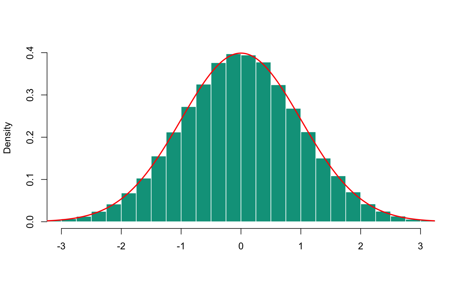
Figure 16.1: Histogram of simulated normal sample
x <- rnorm(n, mu=0, sigma=1)16.4.3 Lognormal Distribution
Simulating a log-normal distribution \(\mathcal{LN}or(\mu,\sigma^2)\) is done based on the simulation of a normal distribution \(\mathcal{N}or(\mu,\sigma^2)\): \(Y = \exp(X)\), where \(X \sim \mathcal{N}or(\mu,\sigma^2)\).
x <- rlnorm(n)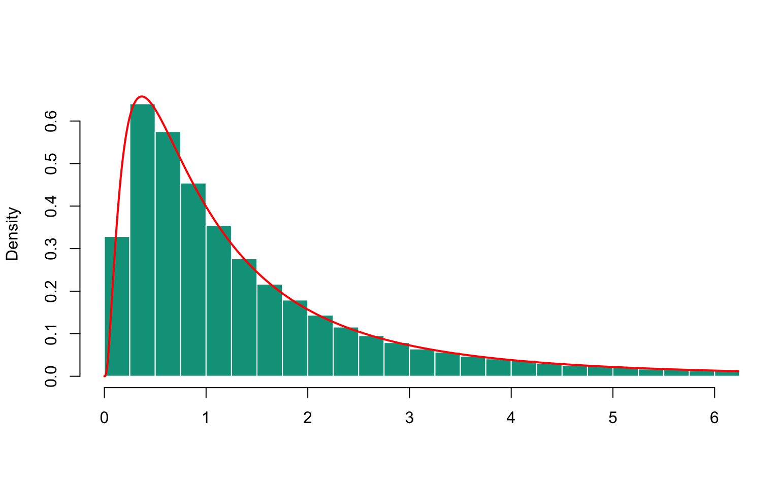
Figure 16.2: Histogram of simulated lognormal sample
16.4.4 Gamma Distribution
Using the results from Section 2.5.7 of Volume 1 regarding the Gamma distribution, it is possible to simulate it without too much difficulty using rejection methods. However, it should be noted that if \(X \sim \mathcal{G}am(a_X,b)\) and \(Y \sim \mathcal{G}am(a_Y,b)\) are independent, then \(X+Y \sim \mathcal{G}am(a_X+a_Y,b)\). The \(\mathcal{G}am(n,b)\) distribution for \(n\in\mathbb{N}\) can be simulated as the sum of \(n\) independent \(\mathcal{E}xp(b)\) variables. More precisely,
Algorithm: Exponential random variable
- \(X \leftarrow -b\log\left(\texttt{Random}\right)\)
Algorithm: Gamma Distribution Simulation \(\mathcal{G}am(a,1)\) where \(a\in \mathbb{N}\)
- \(i \leftarrow 1\) and \(Z \leftarrow 0\)
- Repeat
- \(Z \leftarrow Z - \log \left( \texttt{Random}\right)\)
- \(i \leftarrow i + 1\)
- Until \(i > \alpha\)
For a more general approach (with \(a\) not necessarily an integer), without loss of generality, we assume that \(b=1\). Indeed, if \(X\) follows a \(\mathcal{G}am(a_X, b)\) distribution, then \(Y = bX\) follows a \(\mathcal{G}am(a_Y, b)\) distribution. The challenge lies in simulating \(\mathcal{G}am(a, 1)\) distributions. Two algorithms can be used depending on the relationship between \(a\) and \(1\) (see (Devroye 1992) or (Fishman 2013)):
- If \(0 < a < 1\), and denoting \(e\) as the exponential of \(1\), we can use a rejection method based on \[ g(x) = \frac{ae}{a+e}\left(x^{a-1}\mathbb{I}[0 < x < 1]+\exp(-x)\mathbb{I}[1 \leq x]\right). \] A variable with such a density can be easily simulated using the inversion algorithm, as the quantile function is given by \[\begin{eqnarray*} G^{-1}(u) &=& \left(\frac{a+e}{e}u\right)^{1/a}\mathbb{I}[0 < x < e/(a+e)]\\ && - \log\left(\frac{a+e}{ae}(1-u)\right)\mathbb{I}[e/(a+e) \leq x]. \end{eqnarray*}\]
To simulate realizations of the \(\mathcal{G}am(a, 1)\) distribution, the Ahrens-Dieter algorithm is used, as shown below:
Algorithm: Ahrens-Dieter Algorithm
- \(\texttt{test}\leftarrow 0\) and \(A\leftarrow\left[(a-1) - 1/6(a-1)\right] / (a-1)\)
- Repeat \(X \leftarrow (a+e)/e \times \texttt{Random}\)
- If \(X \leq 1\) Then \(Z \leftarrow X^{1/a}\),
- If \(Z \leq -\log \left(\texttt{Random}\right)\) Then \(\texttt{test}\leftarrow 1\)
- If \(X > 1\) Then \(Z \leftarrow -\log \left(\left((a+e)/e-X\right)/a\right)\)
- If \(Z \geq \texttt{Random}^{1/(a-1)}\) Then \(test\leftarrow 1\)
- If \(X \leq 1\) Then \(Z \leftarrow X^{1/a}\),
- Until \(\texttt{test}\leftarrow 1\)
- If \(a > 1\) and is not an integer, the Cheng-Feast algorithm can be used:
Algorithm: Cheng-Feast Algorithm
- \(\texttt{test}\leftarrow 0\) and \(A\leftarrow\left[(a-1) - 1/6(a-1)\right] / (a-1)\)
- Repeat
- \(U \leftarrow \texttt{Random}\)
- \(V \leftarrow \texttt{Random}\)
- \(X \leftarrow A \times U/V\)
- If \(2U/a-(2/a+2)+X+1/X \leq 0\) Then \(\texttt{test}\leftarrow 1\)
- Until \(\texttt{test}\leftarrow 1\)
- \(Z \leftarrow aX\)
16.4.5 Beta Distribution
To simulate a Beta distribution with parameters \(\alpha\) and \(\beta\) (see Section 2.5.3 for properties of the Beta distribution), the following result, known as Jöhnk’s Theorem, is used:
Proposition 16.1 Let \(U\) and \(V\) be two independent variables following \(\mathcal{U}ni(0,1)\). For positive \(a\) and \(b\), let \(S=U^{1/a}/\left(U^{1/a}+V^{1/b}\right)\). Then, \(S\), conditioned on \(T=U^{1/a}+V^{1/b}\leq 1\), follows a Beta distribution with parameters \(a\) and \(b\).
Proof. Note that \(X=U^{1/a}\) has a cumulative distribution function \(x^a\) on \([0,1]\), and its probability density function is \(x\mapsto ax^{a-1}\). Similarly, for \(Y=V^{1/b}\), the probability density function is \(y\mapsto by^{b-1}\). Thus, the joint density of the pair \((X,Y)\) is given by \[ f(x,y) = abx^{a-1}y^{b-1} \text{ for } (x,y) \in [0,1] \times [0,1]. \] By considering the change of variables \((s,t) = (x+y,x/(x+y))\), which inverses to \((x,y) = (st,s(1-t))\), we can easily derive the density of the pair \((S,T)\), which takes the form \[ (s,t) = abt^{a-1}(1-t)^{b-1}s^{a+b-1} \] for \((s,t) \in \{(x,y)|y>0,0<x<\min\{1/y,1/(1-y)\}\}\). Thus, the density of \(T\) is given by \[ t\mapsto \frac{1}{\kappa}\frac{ab}{a+b}t^{a-1}(1-t)^{b-1} \text{ for } t \in [0,1], \] where \(\kappa\) is a normalization constant. Consequently, \(T\) follows a Beta distribution with parameters \(a\) and \(b\).
From this, we can derive the following algorithm:
Algorithm: Jöhnk Generator
- Repeat
- \(U\Leftarrow \texttt{Random}^{1/a}\)
- \(V\Leftarrow \texttt{Random}^{1/b}\)
- Until \(U+V \leq 1\)
- \(S\leftarrow U/\left( U+V\right)\) ******
u <- runif(n)^(1/a)
v <- runif(n)^(1/b)
idx <- ((u+v)<=1)
s <- (u/(u+v))[idx]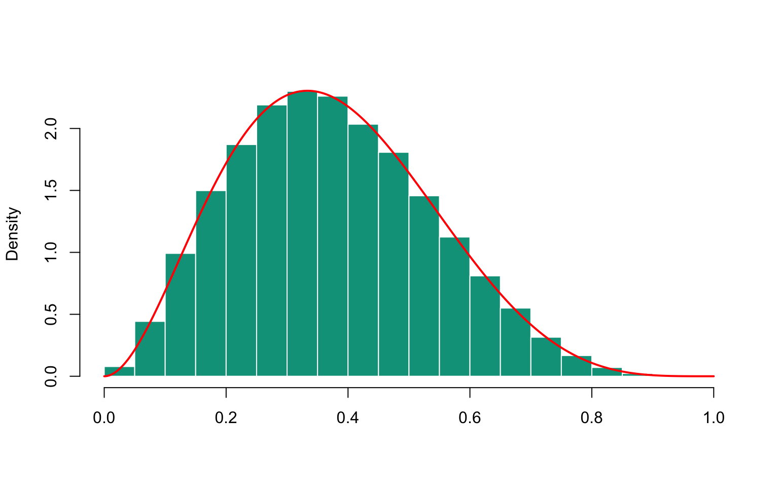
Figure 16.3: Histogram of simulated beta sample
16.4.6 Poisson Distribution
For several probability distributions we will discuss subsequently, probabilities generally involve calculations of factorials. If we want to simulate the number of claims in a relatively large portfolio following a Poisson distribution, the probability of having 20 claims would involve 20!, which, as a reminder, is of the order of \(10^{18}\). For some calculations, it may be necessary, to avoid zero probabilities, to approximate factorials.
Example 16.12 Several relationships can be used to approximate \(n!\) when \(n\) is large, among which the most commonly used is Stirling’s formula: \[ \log n! \thickapprox \left( n+\frac{1}{2}\right) \log \left(n+1\right) - \left(n+1\right) + \frac{1}{2}\log \left(2\pi\right). \] More precisely, using Binet’s series, we have the following inequalities: \[ \left( n+\frac{1}{2}\right) \log \left( n+1\right) - \left(n+1\right) + \frac{1}{2}\log \left( 2\pi \right) \leq \log n! \] and \[ \log n! \leq \left( n+\frac{1}{2}\right) \log \left( n+1\right) - \left(n+1\right) +\frac{1}{2}\log \left( 2\pi \right) +\frac{1}{12\left(n+1\right) }. \]
16.4.7 Poisson Distribution
In Chapter 7 of Volume 1, we saw that a Poisson process consists of durations separating two successive events that are independent and exponentially distributed with a parameter \(\lambda\). In other words, if \(\{ T_1, T_2, \ldots \}\) is a sequence of independent \(\mathcal{Exp}(\lambda)\) random variables, the distribution of \[\begin{eqnarray*} N_{t} &=& \sum_{n\geq 1} n \mathbb{I}\big[ T_{1}+T_{2}+\ldots+T_{n} \leq t < T_{1}+T_{2}+\ldots+T_{n}+T_{n+1}\big]\\ &\sim& \mathcal{P}oi(\lambda t). \end{eqnarray*}\] To simulate a Poisson distribution with parameter \(\lambda\), we use the fact that \(-\log U/\lambda\) follows an exponential distribution with parameter \(\lambda\). Therefore, if \(\{ U_1, U_2, \ldots \}\) is a sequence of independent random variables following a \(\mathcal{U}ni(0,1)\) distribution, \[\begin{equation*} X = \sum_{n\geq 1} n \mathbb{I}\big[ U_{1}U_{2}\ldots U_{n}U_{n+1} \leq e^{-\lambda} < U_{1}U_{2}\ldots U_{n}\big] \sim \mathcal{P}oi(\lambda). \end{equation*}\] Hence, the following algorithm:
Algorithm: xxxxxx
- \(X\longleftarrow -1\), \(P\longleftarrow 1\)
- Repeat
- \(X\longleftarrow X+1\), \(Q=P\)
- \(P\longleftarrow P\times \mathtt{Random}\)
- Until \(P\leq \exp \left( -\lambda \right)<Q\)
Remark. For relatively large values of \(\lambda\), it may be interesting to approximate the Poisson distribution with the normal distribution.
x <- rpois(n, lambda = 1)16.4.8 Geometric Distribution
To simulate a geometric distribution with parameter \(p\), we will use the following result:
Lemma 16.2 If \(X\) follows an exponential distribution with parameter \(-1/\log p\), then \([X]\) follows the geometric distribution with parameter \(p\), where \([\cdot]\) denotes the floor function.
Proof. Let \(Y=[X]\) be the floor of \(X\), where \(X\sim\mathcal{Exp}\left(-1/\log p\right)\). Then, for \(k\in \mathbb{N}\), we can write \[\begin{eqnarray*} \Pr[Y=k] &=& \Pr\left[ k\leq X<k+1\right]\\ &=& F_X\left(k\right) - F_X\left(k+1\right)\\ &=& \exp \left( \left( k+1\right) \log p\right) - \exp \left( k\log p\right)\\ &=& \left( 1-p\right)p^{k}, \end{eqnarray*}\] which gives the desired result.
From this result, we derive the following algorithm:
Algorithm: xxxxxx
- $X() $
16.4.9 Binomial Distribution
By definition, the Binomial distribution counts the number of successes of an event with a probability \(p\) of occurring in \(n\) trials. The \(\mathcal{B}in(n, p)\) distribution can be viewed as the sum of \(n\) random variables with a \(\mathcal{B}in(1, p)\) distribution. The simplest algorithm is as follows:
Algorithm: xxxxxx
- \(X\longleftarrow 0\) \(\mathtt{et}\) \(i\Longleftarrow 0\)
- Repeat
- \(X\longleftarrow X+\boldsymbol{1}(\mathtt{Random}\leq p)\)
- \(i\longleftarrow i+1\)
- Until \(i=n\)
However, note that this algorithm can be relatively slow if \(n\) is large (the time to obtain one realization is then proportional to \(n\)). Two other algorithms can be used, thanks to the following result,
Proposition 16.2 (Waiting Times)
- Let \(G_{1},G_{2},...\) be independent \(\mathcal{G}eo(p)\) variables, and let \(X\) be the smallest integer such that \(G_{1}+...+G_{X+1}>n\). Then \(X\sim\mathcal{B}in(n,p)\).
- Let \(E_{1},E_{2},...\) be independent \(\mathcal{E}xp(1)\) variables, and let \(X\) be the smallest integer such that \[ \frac{E_{1}}{n}+\frac{E_{2}}{n-1}+\frac{E_{3}}{n-2}+...+\frac{E_{X+1}}{n-X} >-\log \left( 1-p\right). \] Then \(X\sim\mathcal{B}in(n,p)\).
Proof. The first result can be verified directly or by noting that $G_{1} eo( p) $ corresponds to the number of draws needed before obtaining the first success, \(G_{2}\) corresponds to the additional draws needed before obtaining the second success, and so on.
To prove the second result, let \(X_{1},...,X_{n}\) be independent random variables, all with the same $xp( ) $ distribution. Define \(X_{1:n} \leq X_{2:n } \leq \ldots \leq X_{n:n }\) as the order statistics, and let \(Z_{1}=X_{1:n}\), $Z_{2}=X_{2:n }-X_{1:n} $, …, \(Z_{n}=X_{n:n }-X_{n-1:n }\). We will show that the variables \(Z_{k}\) are independent and have an \(\mathcal{E}xp\left( (n-k+1) \alpha \right)\) distribution.
The joint density of $(X_{1:n},…,X_{n:n}) $ is given by: \[\begin{equation*} f\left( y_{1},...,y_{n}\right) =n!\alpha ^{n}\exp \left( -\alpha \left( y_{1}+...y_{n}\right) \right)\mathbb{I}[0<y_{1}<...<y_{n}]. \end{equation*}\]
To obtain the distribution of the vector ${}=( Z_{1},…,Z_{n})^t $, we consider an application \(h:{\mathbb{R}}^{n}\rightarrow \mathbb{R}\) that is a positive Borel function, and write: \[\begin{eqnarray*} \mathbb{E}[ h\left( \boldsymbol{Z}\right) ] &=&\int_{{\mathbb{R}}^{n}}h\left( \boldsymbol{z}\right) dF_{\boldsymbol{Z}}\left( \boldsymbol{z}\right)\\ &=&\int_{{\mathbb{R}}^{n}}h\left( y_{1},y_{2}-y_{1},...,y_{n}-y_{n-1}\right) f\left( y_{1},...,y_{n}\right) dy_{1}...dy_{n} \\ &=&\int_{{\mathbb{R}}^{n}}h\left( y_{1},y_{2}-y_{1},...,y_{n}-y_{n-1}\right) \\ &&n!\alpha ^{n}\exp \left( -\alpha \left[ y_{1}+...y_{n}\right] \right) \mathbb{I}[0<y_{1}<...<y_{n}]dy_{1}...dy_{n}. \end{eqnarray*}\]%
We then introduce the change of variables: \[\begin{equation*} \left\{ \begin{array}{rcl} y_{1} & = & z_{1} \\ y_{2}-y_{1} & = & z_{2} \\ & & \\ y_{n-1}-y_{n-2} & = & z_{n-1} \\ y_{n}-y_{n-1} & = & z_{n}% \end{array}% \right. \text{ or }\left\{ \begin{array}{rcl} y_{1} & = & z_{1} \\ y_{2} & = & z_{1}+z_{2} \\ & & \\ y_{n-1} & = & z_{1}+z_{2}+...+z_{n-1} \\ y_{n} & = & z_{1}+z_{2}+...+z_{n-1}+z_{n}% \end{array}% \right. \end{equation*}\]% with a Jacobian of 1. The expectation of $h( ) $ can then be written as: \[\begin{equation*} \mathbb{E}[ h\left( \boldsymbol{Z}\right) ] =n!\alpha ^{n}\int_{{\mathbb{R}}^{n}}h\left( \boldsymbol{z}\right) \exp \left( -\alpha \sum_{i=1}^n(n-i+1)z_i \right) dz_{1}...dz_{n} \end{equation*}\]%
This gives us the density of the vector \(\boldsymbol{Z}\): \[\begin{eqnarray*} f_{ \boldsymbol{Z}}(\boldsymbol{z}) &=&n!\alpha ^{n}\exp \left( -\alpha \sum_{i=1}^n(n-i+1)z_i \right) \\ &&\mathbb{I}[z_{1}>0,z_{2}>0,...,z_{n}>0] \\ &=&\prod_{k=1}^{n}f_{k}\left( z_{k}\right) \end{eqnarray*}\] where \[ f_{k}\left( z_{k}\right) =\alpha \left( n-k+1\right) \exp \left( -\left( n-k+1\right) \alpha z_{k}\right) \cdot\mathbb{I}[z_{k}>0]. \]
We can observe that in this form, the \(f_{k}\) functions are densities, and they correspond to the densities of \(Z_{k}\). Therefore, the variables \(Z_{k}\) are independent and have an $xp(( n-k+1)) $ distribution, as claimed.
This allows us to conclude that $ ( E_{1:n},E_{2:n},…,E_{n:n}) $ \[ =_{\text{loi}}\left( \frac{E_{1}}{n},% \frac{E_{1}}{n}+\frac{E_{2}}{n-1},...,\frac{E_{1}}{n}+\frac{E_{2}}{n-1}+...+% \frac{E_{n-1}}{2}+E_{n}\right) . \]
Furthermore, the number of \(E_{i}\) among the \(n\) that are less than $-( 1-p) $ follows a binomial distribution with parameters \(n\) and% \[ \Pr\left[ E_{1}\leq -\log \left( 1-p\right) \right] =1-\exp \left( \log \left( 1-p\right) \right) =p. \]%
This concludes the proof.
The simulation algorithms are as follows,
Algorithm: xxxxxx
- \(X\longleftarrow -1\), \(S\longleftarrow 0\)
- Repeat
- \(S\longleftarrow S+Int(\log(\mathtt{Random})/(1-p))\)
- \(X\longleftarrow X+1\)
- Until \(S>n\)
or, in the second case,
Algorithm: xxxxxx
- \(X\longleftarrow 0\), \(S\longleftarrow 0\)
- Repeat
- \(S\longleftarrow S-\log(\mathtt{Random})/(n-X)\)
- \(X\longleftarrow X+1\)
- Until \(S>-\log(1-p)\)
(for the latter algorithm, it is \(X-1\) that will follow the binomial distribution). These two algorithms can be relatively efficient because the time is proportional to \(np+1\).
16.4.10 Negative Binomial Distribution
The simulation algorithms for the negative binomial distribution are as follows:
Algorithm: xxxxxx
- \(X\longleftarrow -1\) and \(S\longleftarrow 0\)
- Repeat
- \(S\longleftarrow S+\text{Int}(\log(\text{Random})/(1-p))\)
- \(X\longleftarrow X+1\)
- Until \(S>n\)
Or, in the second case:
Algorithm: xxxxxx
- \(X\longleftarrow 0\), \(S\longleftarrow 0\)
- Repeat
- \(S\leftarrow S-\log(\text{Random})/(n-X)\)
- \(X\longleftarrow X+1\)
- Until \(S>-\log(1-p)\)
(In the latter algorithm, it’s \(X-1\) that follows the binomial distribution.) These two algorithms can be relatively efficient because the time complexity is proportional to \(np+1\).
16.4.11 Negative Binomial Distribution
To simulate a negative binomial distribution, the following algorithm can be used:
Algorithm: xxxxxx
- $Y\(\texttt{Gamma Distribution }\)am(n,1)$
- $X$ \(\mathcal{P}oi(Y/(1-p))\)
Example 16.13
In dimension \(2\), one can simulate a Gaussian vector as follows: \[\begin{equation*} \left( \begin{array}{c} X \\ Y% \end{array}% \right) \sim \mathcal{N}or\left( \left( \begin{array}{c} \mu _{X} \\ \mu _{Y}% \end{array}% \right) ,\left( \begin{array}{cc} \sigma _{X}^{2} & r\sigma _{X}\sigma _{Y} \\ r\sigma _{X}\sigma _{2} & \sigma _{Y}^{2}% \end{array}% \right) \right) , \end{equation*}\] noting that the conditional distribution of \(X\) given \(Y=y\) is Gaussian, i.e., \[\begin{equation*} [ X|Y=y] \sim \mathcal{N}or\left( \mu _{X}+r\frac{\sigma _{X}}{% \sigma _{Y}}\left( y-\mu _{Y}\right) ,\sigma _{X}^{2}-r^{2}\sigma _{Y}^{2}\right) . \end{equation*}\] The algorithm is as follows:16.4.12 Elliptical Distributions
Elliptical distributions (discussed in Section 2.6.5 of Volume 1) can be easily simulated from their canonical representation. Recall that a random vector \(X\) follows an elliptical distribution \(\mathcal{Ell}(g,\boldsymbol{\mu},\boldsymbol{\Sigma})\) if, and only if, \[ {\boldsymbol{X}}\stackrel{\text{law}}{=} {\boldsymbol{\mu}}+R{\boldsymbol{A}}^t{\boldsymbol{U}}, \] where \({\boldsymbol{A}}^t{\boldsymbol{A}}=\mathbf{\Sigma}\), and \(R\) is an independent random variable of \(\boldsymbol{U}\), with \(\boldsymbol{U}\) uniformly distributed on the unit sphere in \(\mathbb{R}^n\) (see (Fang and Kotz 1990)). The law of \(R\) depends on the generator. Therefore, to simulate an elliptical vector, one simply needs to simulate \(R\), and then simulate (independently) a uniform distribution on the unit sphere.
Example 16.14 The Gaussian vector is a particular elliptical vector, where \(R^2\) follows a chi-squared distribution. Therefore, we can use an algorithm similar to the one for simulating two independent Gaussian variables. To simulate a vector \(Z\) uniformly distributed on the sphere of radius \(r\) in \(\mathbb{R}^d\), \[\begin{equation*} \mathcal{S}=\left\{ \mathbf{z}\in\mathbb{R}^d|z_{1}^{2}+...+z_{d}^{2}=r^{2}\right\}, \end{equation*}\] with density given by \[\begin{equation} f\left( \mathbf{z}\right) =\frac{\Gamma \left( d/2\right) }{\left( 2\pi \right) ^{d/2}r^{d-1}},\qquad \mathbf{z}\in \mathcal{S}, \tag{16.1} \end{equation}\] we note that if \(\mathbf{X}\sim\mathcal{Nor}(\boldsymbol{0},\mathbf{I})\), and if we let \(W=\sqrt{X_{1}^{2}+...+X_{d}^{2}}\), then the vector \(\mathbf{Z}\), where \(Z_{i}=X_{i}/W\) for \(i=1,...,d\), follows the density in Equation (16.1). Hence, the algorithm is as follows:
Algorithm: Simulating Uniform Distribution on the Sphere
- \(i\Longleftarrow 0\) and \(W\Longleftarrow 0\)
- Repeat
- \(i\longleftarrow i+1\)
- \(X_{i}\Longleftarrow\cos\left( 2\pi \times \mathtt{Random}\right)\sqrt{-2\log\mathtt{Random}}\)
- \(W\Longleftarrow W+X_{i}\)
- Until \(i=n\)
16.4.13 Using Copulas
As mentioned earlier, one method to simulate pairs of random variables is to use conditional distributions. The idea, generally attributed to (Rosenblatt 1952), is to use the following algorithm:
- Simulate \(Y\) following \(F_{Y}\).
- Then, simulate \(X|Y\) following \(F_{X|Y}\).
However, it is also possible to transform the margins into pairs that can be easily simulated through transformations. The idea is to find transformations \(\phi\) and \(\psi\) such that the pair \(\left( \phi(X), \psi(Y)\right)\) is simulatable. In particular, it is possible to generate Gaussian vectors and all families of distributions derived from them.
To simulate random vectors \(\left( X, Y\right)\) with marginal distribution functions \(F_{X}\) and \(F_{Y}\), it is possible to simulate the associated vector \(\left( U, V\right)\) with copula \(C\). Then, by inverting the marginal distribution functions, \(\left( F_{X}^{-1}\left( U\right), F_{Y}^{-1}\left( V\right)\right)\) will have marginal distribution functions \(F_{X}\) and \(F_{Y}\) and copula \(C\) (the theory of copulas is discussed in detail in Section 8.6 of Volume 1).
Example 16.15 To simulate \((U,V)\) from the Clayton copula with parameter \(\alpha\) (defined in equation (8.22)), we use Example 8.6.8, which provides the following algorithm:
Algorithm: xxxx
- \(U\longleftarrow\mathtt{Random}\) and \(T\Longleftarrow\mathtt{Random}\)
- \(V\longleftarrow [(T^{-\theta /(1+\theta )}-1)U^{-\theta}+1]^{-1/\theta }\)
This method, presented here in dimension \(2\), can nonetheless be generalized to higher dimensions.
16.5 Simulation of Stochastic Processes
In many cases, it is not sufficient to simulate random variables, and the simulation of a process is required (for example, in Chapter 7 of Volume 1, for calculating ruin probabilities). A process corresponds to a sequence of random variables. Simulating a process is, therefore, equivalent to simulating a sequence of random variables.
16.5.1 Simulation of Markov Chains
Markov chains were used in Chapter 11 to model the trajectory of an insured person in a bonus-malus scale. Heuristically, a Markov chain is a sequence of random variables for which the best prediction that can be made at time \(n\) for future times, given all previous values up to time \(n\), is identical to the prediction made if only the value at time \(n\) is known, i.e., \[\begin{equation*} \left[ X_{n+1}|X_{n}=x_{n},X_{n-1}=x_{n-1},...\right] \stackrel{\text{law}}{=}\left[ X_{n+1}|X_{n}=x_{n}\right]. \end{equation*}\] Equivalently, a Markov chain \(\{X_0,X_1,X_2,\ldots\}\) is a sequence of random variables taking values in a space \(E\) such that there exists a sequence \(\{U_0,U_1,U_2,\ldots\}\) of independent random variables and a measurable function \(h\) such that \[\begin{equation*} X_{n+1}=h_n \left(X_{n},U_{n}\right), \text{ for all } n\in \mathbb{N}. \end{equation*}\] In the case where this transformation does not depend on \(n\), we say that the chain is homogeneous. Simulating a trajectory of the Markov chain \(\{X_0,X_1,X_2,\ldots\}\) involves, starting from a known \(X_0\), generating \(U_0,U_1,\ldots\) to compute \(X_1=h(X_0,U_0)\), \(X_2=h(X_1,U_1)\), and so on.
Example 16.16 Consider the case of a random walk. Let \(\{U_0,U_1,U_2,\ldots\}\) be a sequence of independent random variables, and define the sequence \(\{X_0,X_1,X_2,\ldots\}\) of variables by \[\begin{equation*} X_{n+1}=X_{n}+U_{n},\hspace{3mm} n\in \mathbb{N}. \end{equation*}\] A special case is when \(X_{0}\) is an integer, and \(\Pr\left[ U_{n}=-1\right] =\Pr\left[ U_{n}=+1\right] =1/2\), corresponding to the coin toss game.
16.5.2 Simulation of a Poisson Process
Continuous-time processes are difficult to simulate because from a numerical point of view, continuous time does not exist. However, simulating a Poisson process is a special case. In general, consider a Poisson process with intensity function $( t) $ (Section 7.3.1 of Volume 1 presented the main results concerning these processes). The idea is to simulate \(T_1\), the time of the first event, and then iteratively calculate the distribution of the time between the \((i+1)\)-th and \(i\)-th events, given that the \(i\)-th event occurred at time \(T_i\). For this purpose, recall that for \(s<t\), \(N_t-N_s\) follows a Poisson distribution with parameter \(\Lambda(t)-\Lambda(s)\), where \[ \Lambda(t)=\int_{[0,t]}\lambda(s)ds. \]
Example 16.17 Consider a Poisson process with intensity function $( t) =1/( t+a) $ for \(t\geq 0\), where \(a\) is a positive constant. Then, \[\begin{equation*} \int_{0}^{x}\lambda \left( s+y\right) dy=\log \left( \frac{x+s+a}{s+a} \right). \end{equation*}\] The cumulative distribution function of the time between two successive events, given that an event occurred at time \(s\), is \[ \Pr\left[ \text{Time to Next Event}\leq x|\text{Event at }% s\right] \] \[ =\frac{x}{x+s+a} \] which can be easily inverted. The simulation algorithm for such a process is as follows:
Algorithm: xxxx
- $U\(\texttt{Random and }\)i=1$
- \(T_{1}\Longleftarrow a\times U/(1-U)\)
- Repeat \(i\longleftarrow i+1\)
- \(U\longleftarrow \texttt{Random}\)
- \(T_{i}\longleftarrow \left(T_{i-1}+a\right) \times U/(1-U)\)
16.5.3 Calculating Ruin Probability through Simulation
16.5.3.1 The Problem
In Chapter 7, we presented classical results related to the calculation of ruin probability. Let’s revisit this problem and focus on the process corresponding to the company’s result: \[ R_t=\kappa+ct-S_t=\kappa+ct-\sum_{i=1}^{N_t}X_i, \] where \(c\) is the premium rate, and \(\kappa\) is an initial capital. We assume that \(S_t\sim\mathcal{CP}oi(\lambda t,F)\). We will assume that \(F\) has a finite mean \(\mu\). Figure ?? presents simulations of \(6\) trajectories of such a process over \(25\) years.
FIG
The ruin time of the insurance company is defined as the stopping time: \[ T=\inf\{t\geq0| R_t<0\}=\inf\{t\geq0| S_t>\kappa+ct\}. \] We define the probability of ultimate ruin as: \[ \psi(\kappa)=\Pr[T<\infty|R_0=\kappa], \] and the finite-time ruin probability (\(\tau\)) as: \[ \psi(\kappa,\tau)=\Pr[T<\tau|R_0=\kappa]. \] Apart from a few simple cases where these probabilities can be calculated without much difficulty, their evaluation is generally challenging. We show here how to estimate them through simulation.
16.5.3.1.1 Standard Monte Carlo Method for Finite-Time Ruin Probability
For such a process, note that ruin can only occur at an event occurrence time (see Section 7.3.4 for a connection with de Finetti’s discrete model). In particular, we have seen that \[ \psi(\kappa)=\Pr\left[\sum_{j=0}^i\Delta_j>\kappa \text{ for some }i\Big|R_0=\kappa\right], \] where the variables \(\Delta_1,\Delta_2,...\), defined by \[ \Delta_j=X_j-c(T_j-T_{j-1}), \] are independent and identically distributed. It is sufficient to simulate the claim amounts \(X_j\) and the event occurrence times \(T_j\). Since we cannot simulate an infinite number of variables, we will focus on the finite-time ruin probability \(\tau\) by simulating event occurrence times \(T_j\) until \(T_j<\tau\). We then simulate a large number of variables \(Z=\mathbb{I}[T>\tau]\) using the following algorithm:
Algorithm: xxxx
- \(T\Longleftarrow 0\),
- \(S\Longleftarrow 0\),
- \(Z\Longleftarrow 0\)
- Repeat \(i\longleftarrow i+1\)
- \(U\Longleftarrow T-\log\left(\mathtt{Random}\right) /\lambda\)
- \(X\longleftarrow\texttt{cost distribution}\)
- \(D\longleftarrow X-c(T_j-T_{j-1})\),
- \(S\longleftarrow S+D\)
- \(T\longleftarrow U\)
- If \(S>\kappa\) Then \(Z\longleftarrow1\)
- Until \(T\geq\tau\) or \(Z=1\)
16.5.3.1.2 Using the Pollaczeck-Khinchine-Beekman Formula for Infinite-Time Ruin Probability
In Remark 7.3.15, we saw that the infinite-time ruin probability can be expressed as \[ \psi(\kappa)=\Pr[M>\kappa], \text{ where }M=\max_{t\geq0}\{S_t-ct\}=L_1+...+L_K, \] where \(K\sim\mathcal{Geo}(q)\), with \(q=1-\psi(0)=1-\lambda\mu/c\), and the variables \(L_i\) are defined iteratively. It can be shown that these variables are independent, and the distribution of \(L_i\) is \(\tilde{F}\), defined as in Theorem 7.3.13 by \[ \tilde{F}(x)=\int_{y=0}^{x}\frac{\overline{F}(y)}{\mu}dy, \hspace{3mm}x>0. \] It is then possible to simulate a large number of variables \(Z=\mathbb{I}[T>\tau]\) using the following algorithm:While this method offers a relatively elegant algorithm for approaching infinite horizon scenarios, it is worth noting that the algorithm can be relatively inefficient for large values of \(\kappa\).
16.6 Monte Carlo via Markov Chains
16.6.1 Principle
Similar to Chapter 11, we consider a finite state space \(E\), which we will assume to be \(\left\{ 1,2,...,N\right\}\). The process \(\{X_1,X_2,\ldots\}\) is a Markov chain if the equality \[ \Pr\left[ X_{n+1}=j|X_{n}=i,X_{n-1}=x_{n-1},...,X_{1}=x_{1}\right] \] \[ =\Pr\left[ X_{n+1}=j|X_{n}=i\right], \] holds for all \(i,j\). The Markov chain is characterized by its transition matrices \(\boldsymbol{Q}_n\), of dimension \(N\times N\), such that \[\begin{equation*} Q_{n}\left( i,j\right) =\Pr\left[ X_{n+1}=j|X_{n}=i\right] \end{equation*}\] and its initial distribution \(\mu \left( i\right) =\Pr\left[ X_{0}=i\right]\). Here, we only consider the case of homogeneous Markov chains, i.e., the transition matrix is time-invariant, i.e., $Q_{n}( i,j) =Q( i,j) $ for all \(n\).
To simulate a Markov chain, we set the initial value to \(X_{0}=i\), then use the following algorithm:
Algorithm: xxxx
- \(n\Longleftarrow 0\)
- \(X_{0}\Longleftarrow i\) (initial state)
- Repeat
- \(n\longleftarrow n+1\)
- \(p\longleftarrow 0,\) \(j=1,1\)
- \(U\longleftarrow \mathtt{Random}\)
- Repeat
- $pp+Q(i,j) $
- \(j\longleftarrow j+1\)
- Until \(U>p\)
- \(X_{n}\longleftarrow j-1\)
The distribution of \(X_{n}\) is then given by \[\begin{equation*} \Pr\left[ X_{n}=j\right] =\sum_{i=1}^{N}\mu _{i}Q^{n}\left( i,j\right) \end{equation*}\] where \(\mu_i=\Pr[X_0=i]\), and \(\boldsymbol{Q}^{n}\) denotes the \(n\)th matrix power of \(\boldsymbol{Q}\), which satisfies the Chapman-Kolmogorov equation: \[\begin{equation*} Q^{n+1}\left( i,j\right) =\sum_{k=1}^{N}Q\left( i,k\right) Q^{n}\left( k,j\right). \end{equation*}\]
A probability distribution \(\boldsymbol{\mu}\) (represented by the vector \((\mu_1,\ldots,\mu_N)^t\) of probability masses assigned to \(1,\ldots,N\)) satisfying \(\boldsymbol{\mu}=\boldsymbol{\mu}\boldsymbol{Q}\) is called an invariant distribution associated with the Markov chain. Therefore, to simulate a random variable with distribution \(\boldsymbol{\mu}\), one can look for a family of Markov chains with an invariant measure \(\boldsymbol{\mu}\) (because under certain conditions, the distribution of \(X_{n}\) “converges” to \(\boldsymbol{\mu}\)). Among the conditions allowing this convergence, we will retain the following two notions:
- A Markov chain is called irreducible if one can go from any point in \(E\) to any other point in \(E\) with a non-zero probability, i.e., there exists \(n\) such that \[ \Pr[X_{0}=i,X_{n}=j] =Q^{n}\left( i,j\right) >0 \] for all \(i,j\).
- A Markov chain is called aperiodic if there exists a state \(j\) and an integer \(n\) such that \(Q^{n}\left( j,j\right) >0\) and \(Q^{n+1}\left( j,j\right) >0\). \end{enumerate}
In the case where the state space \(E\) is finite, and if the Markov chain is irreducible and aperiodic, with an invariant measure \(\boldsymbol{\mu}\), then there exist \(M\) and \(c\) such that \[\begin{equation*} \left| Q^{n}\left( i,j\right) -\mu_j \right| \leq M\exp \left( -cn\right) . \end{equation*}\]
In this case, there is an exponential convergence rate towards the limit distribution.
16.6.2 Some Notions of Ergodic Theory
The central idea behind using Markov chains for Monte Carlo methods is to start from an initial value \(X_{0}\) and then generate a Markov chain whose limiting distribution is \(f\), the density we want to simulate. After a certain number \(T\) of iterations, we can assume that we have reached a steady state, and we can then consider that \(X_{T}\) has density \(f\). A non-independent sample is then obtained by considering \(X_{T+1},...,X_{T+n}\). This lack of independence is generally not a problem for the evaluation of integrals. All that is required is to simulate a sequence of stationary and ergodic variables.
Definition 16.1 A sequence of random variables \(X_1,X_2,...\) is called stationary if \((X_1,...,X_k)=_{\text{law}}(X_{1+h},...,X_{k+h})\) for all \(k,h\geq 0\). Such a sequence is called ergodic if, and only if, for any Borel set \(B\) and any \(k\in\mathbb{N}\), \[ \Pr\left[\frac{1}{n}\sum_{t=1}^n \mathbb{I}_B(X_t,X_{t+1},...,X_{t+k})\rightarrow \Pr[(X_t,X_{t+1},...,X_{t+k})\in B]\right]=1. \]
16.6.2.0.1 Recurrence
In practice, if \(\{X_1,X_2,\ldots\}\) is a Markov chain, several results can be obtained. Among the central concepts, recall the notion of recurrence. For a finite state space, if \(N(x)\) is the number of visits of the chain to state \(x\), then state \(x\) is said to be recurrent if \[ \mathbb{E}[N(x)]=\mathbb{E}\left[\sum_{t=1}^\infty \mathbb{I}[X_t=x]\right]=\infty. \] If the expectation is finite, it is referred to as a transient state.
In the continuous case, we introduce the notion of Harris-recurrent set (or Harris-recurrent in the sense of Harris). By denoting \(N(A)\) as the number of visits to the set \(A\), the set \(A\) is said to be Harris-recurrent if \[ \Pr[N(A)=\infty]=\Pr\left[\sum_{t=1}^\infty \mathbb{I}[X_t\inA]\right] =1. \] The Markov chain will be called Harris-recurrent if every set \(A\) is Harris-recurrent.
From this notion, we can introduce a law of large numbers for non-independent series. A rigorous proof of this result can be found in (Robert 1996).
Proposition 16.3 If a Markov chain \((X_t)\) is Harris-recurrent, then for any \(h\) (such that the expectation exists), \[ \lim_{n\rightarrow\infty}\frac{1}{n}\sum_{i=1}^nh(X_i)=\int h(x)dF(x), \] where \(F\) denotes the cumulative distribution function of the invariant distribution associated with the chain.
16.6.3 Simulation of an Invariant Measure: Hastings-Metropolis Algorithm
Among the Monte Carlo methods by Markov Chain (MCMC), we note the Hastings-Metropolis algorithm, which allows us to simulate an invariant distribution $$. Here, we assume that for every state \(j\), \(\mu_j >0\).
The Hastings-Metropolis algorithm uses an instrumental distribution $q( y|x) $ to simulate the target density \(f\) (referred to as the target density). The iterative algorithm is as follows: starting from \(X_{t}\), we simulate \(Y_{t}\) following the distribution $q( |X_{t}) $, and then we set% \[ X_{t+1}=\left\{ \begin{array}{ll} Y_{t}, & \text{with probability }\pi \left( X_{t},Y_{t}\right) ,\\ X_{t}, & \text{with probability }1-\pi \left( X_{t},Y_{t}\right) ,% \end{array}% \right. \]% where \[ \pi \left( x,y\right) =\min \left\{ \frac{f\left( y\right) }{f\left( x\right) }\frac{q\left( x|y\right) }{q\left( y|x\right) },1\right\} . \]% It is then possible to show that the Markov chain is reversible, i.e., it satisfies \([X_{t+1}|X_{t+2}]=_{\text{law}}[X_{t+1}|X_t]\), indicating that the direction of time has no influence, if \(f\) satisfies the condition known as “detailed balance,” i.e., there exists $K( ,) $ such that for all \(x,y\),% \[ f\left( y\right) K\left( y,x\right) =f\left( x\right) K\left( x,y\right) . \] Under this assumption, for any function \(h\) such that $[| h(X) |] <$, then% \[ \lim_{t\rightarrow \infty }\frac{1}{t}\sum_{i=1}^{t}h\left( X_{i}\right) =\int h\left( x\right) f\left( x\right)dx. \]
The simplest case is when \(q\) is independent of \(x\). Starting from \(X_{t}\), we simulate \(Y_{t}\) following the distribution $q( ) $, and then we set% \[ X_{t+1}=\left\{ \begin{array}{ll} Y_{t}, & \text{with probability }\min \left\{ f\left( Y_{t}\right) q\left( X_{t}\right) /f\left( X_{t}\right) q\left( Y_{t}\right) ,1\right\}, \\ X_{t} ,& \text{otherwise.}% \end{array}% \right. \]% Here, we encounter an algorithm similar to the rejection method presented in Section ??.
Example 16.18 To simulate a Gamma distribution with parameters $$ and $$, where $$ is not an integer, it is possible to combine a rejection method with a simulation of a Gamma distribution with integer parameters. Denoting \(a=[ \alpha ]\) as the integer part of \(\alpha\), we consider the following algorithm:
Algorithm: xxxx
- \(Y\Longleftarrow Gam\left( a,a/\alpha \right) ,\)
- \(X\Longleftarrow Y\) with probability \[ \pi =\big( eY\exp \left( -Y/\alpha \right) /\alpha \big) ^{\alpha -a}. \]
The Hastings-Metropolis algorithm can be written as follows, starting from \(X_{t}\):
Algorithm: xxxx
- \(Y_{t}\Longleftarrow Gam\left( a,a/\alpha \right) ,\)
- \(X_{t+1}\Longleftarrow Y_{t}\) with probability \[ \pi =% \big( Y_{t}\exp \left( \left( X_{t}-Y_{t}\right) \right) /\alpha X_{t}% \big) ^{\alpha -a}, \] and \(X_{t+1}\Longleftarrow X_{t}\) otherwise\(.\)
16.7 Variance Reduction
As we have seen in the introduction, the convergence rate of Monte Carlo methods is \(\sigma /\sqrt{n}\) (Central Limit Theorem). To improve this speed, one can aim to “reduce the variance,” i.e., decrease the value of \(\sigma ^{2}\). Numerous methods exist, with the general idea being to use another representation - in the form of a mathematical expectation - of the quantity to be calculated.
16.7.1 Use of Antithetic Variables
Suppose we want to compute $ =$ where \(U\sim\mathcal{U}ni(0,1)\). Using \(n\) independent uniform variables \(U_{1},...,U_{n}\), the standard Monte Carlo method approximates $$ as% \[\begin{equation*} \theta \approx \frac{1}{n}\Big( h\left( U_{1}\right) +...+h\left( U_{n}\right) \Big) =\widehat{\theta }, \end{equation*}\]% but considering the relationship \[\begin{equation} \int_{0}^{1}h\left( x\right) dx=\frac{1}{2}\int_{0}^{1}\big(h\left( x\right) +h\left( 1-x\right) \big) dx, \tag{16.2} \end{equation}\] we can also approximate $$ using the relation% \[\begin{equation*} \theta \approx \frac{1}{2n}\Big( h\left( U_{1}\right) +h\left( 1-U_{1}\right) +...+h\left( U_{n}\right) +h\left( 1-U_{n}\right) \Big) =% \widehat{\theta }_{A}. \end{equation*}\]% If we denote $X_{i}=h( U_{i}) $ and $Y_{i}=h( 1-U_{i}) $, then% \[\begin{equation*} \mathbb{V}\left[ \widehat{\theta }\right] =\mathbb{V}\left[ \frac{1}{n}\left( h\left( U_{1}\right) +...+h\left( U_{n}\right) \right) \right] =\frac{\mathbb{V}\left[ X\right] }{n} \end{equation*}\] while \[\begin{eqnarray*} \mathbb{V}\left[ \widehat{\theta }_{A}\right] &=&\mathbb{V}\left[ \frac{1}{2n}\left( h\left( U_{1}\right) +h\left( 1-U_{1}\right) +...+h\left( U_{n}\right) +h\left( 1-U_{n}\right) \right) \right] \\ &=&\mathbb{V}\left[ \widehat{\theta }\right] +\frac{\mathbb{C}\left[ X_1,Y_1\right]}{n}. \end{eqnarray*}\]% In other words, $<$ if and only if, \[ \mathbb{C}\left[ h\left( U\right) ,h\left( 1-U\right) \right] <0. \] This condition is satisfied in particular if \(h\) is a monotonic function since \(U\) and \(1-U\) are then negatively dependent by quadrant (as we saw in Section 8.5). Therefore, if \(h\) is a monotonic function, the quality of the approximation is improved.
In general, $=$ can be rewritten as \[ \theta =\mathbb{E}\left[ h\left( F_X^{-1}\left( U\right) \right) \right] =\mathbb{E}\left[ h^{\ast }\left( U\right) \right]\text{ where }h^*=h\circ F_X^{-1}, \] which allows us to reduce it to the uniform case.
Example 16.19 Consider the textbook example (in the sense that the value of $$ is known and equals \(e-1\)) where we want to estimate \(\theta =\mathbb{E}[\exp U]\) with \(U\sim\mathcal{U}ni(0,1)\). Since the function $uh(u) $ is increasing, the use of antithetic variables will reduce the variance. Note that% \[\begin{eqnarray*} \mathbb{C}[\exp U,\exp \left( 1-U\right)] &=&\mathbb{E}[\exp U\exp \left( 1-U% \right)] \\ &&-\mathbb{E}[\exp U]\mathbb{E}[\exp \left( 1-U\right)] \\ &=&e-(e-1)^{2}. \end{eqnarray*}\]% Now, the variance of \(\exp U\) is% \[\begin{equation*} \mathbb{V}[\exp U]=\frac{e^{2}-1}{2}-(e-1)^{2}, \end{equation*}\]% so we can deduce that using a standard simulation scheme leads to% \[\begin{equation*} \mathbb{V}\left[ \exp U\right] \approx 0.2420, \end{equation*}\]% while using antithetic variables results in% \[\begin{eqnarray*} \mathbb{V}\left[ \frac{\exp U+\exp \left( 1-U\right) }{2}\right] &=&\frac{% \mathbb{V}[\exp U]}{2}+\frac{\mathbb{C}[\exp U,\exp \left( 1-U\right)]}{2} \\ &\approx &0.0039, \end{eqnarray*}\] meaning that with the same number of simulations, the variance obtained using antithetic variables is only 1.6% of the variance obtained by a standard Monte Carlo method. The gain in convergence speed can be visualized in Figure ??.
FIG
16.7.2 Use of Control Variates
If $$ (known) represents the mean of the control variable \(Y\), $X+c( Y-) $ is an unbiased estimator of $=% $, and we aim to minimize its variance. It can be noted that the variance is minimized for% \[\begin{equation*} c^{\ast }=-\frac{\mathbb{C}\left[ X,Y\right] }{\mathbb{V}\left[ Y\right]}, \end{equation*}\]% and the variance of $ _{C}=X+c^{}( Y-) $ is then% \[\begin{equation} \mathbb{V}\left[ \widehat{\theta }_{C}\right] =\mathbb{V}[ X] -\frac{% \mathbb{C}\left[ X,Y\right] ^{2}}{\mathbb{V}\left[ Y\right] } \tag{16.3} \end{equation}\]
Example 16.20 Taking Example 16.19 where the goal was to estimate \(\theta =\mathbb{E}[\exp U]\), it can be noted that the use of control variables also reduces the variance. Indeed, consider that% \[\begin{eqnarray*} \mathbb{C}\left[ \exp U,U\right] &=&\mathbb{E}[U\exp U]-\mathbb{E}[\exp U]\mathbb{E% }[U] \\ &=&1-\frac{e-1}{2}. \end{eqnarray*}\]% Equation (16.3) then becomes, for \(X=\exp U\) and $Y=U $% \[\begin{eqnarray*} \mathbb{V}\left[ \widehat{\theta }_{C}\right] &=&\mathbb{V}\left[ X\right] -\frac{% \mathbb{C}\left[ \exp U,U\right] ^{2}}{\mathbb{V}\left[ U\right] } \\ &=&\frac{e^{2}-1}{2}-(e-1)^{2}-12\left( 1-\frac{e-1}{2}\right) ^{3} \\ &\approx &0,0039. \end{eqnarray*}\]% This results in a variance reduction of the same order of magnitude as when using antithetic variables.
16.7.3 Use of Conditioning
Suppose we want to calculate $=[ h(X)] $, and let $Y=h( X) $. Let \(\mathbf{Z}\) be a random vector, and define $V==g() $. Given the relationship% \[\begin{equation*} \mathbb{E}\left[ V\right] =\mathbb{E}\Big[ \mathbb{E}\left[ Y|\mathbf{Z}\right] \Big] =\mathbb{E}\left[ Y\right] \text{,} \end{equation*}\]% we can estimate $=$ by simulating realizations of \(V\). However, for this method to effectively reduce the variance, we need to compare the variances of \(Y\) and \(V\). Using the variance decomposition formula, we see that% \[\begin{eqnarray*} \mathbb{V}[ Y] &=&\mathbb{E}\Big[ \mathbb{V}\left[ Y|\mathbf{Z}\right] \Big] +\mathbb{V}\Big[ \mathbb{E}\left[ Y|\mathbf{Z}\right] \Big] \\ &\geq &\mathbb{V}\Big[ \mathbb{E}\left[ Y|\mathbf{Z}\right] \Big] =\mathbb{V}\left[ V\right] . \end{eqnarray*}\]% In other words, the estimation based on simulations of \(V\) provides better results than simulations of \(Y\) (as long as the simulations are not too complex).
Example 16.21 Let \(A\) and \(B\) be two independent variables, each following exponential distributions $xp( 1) $ and $xp( 1/2) $, respectively. Suppose we want to calculate $=% $. Rewritten in terms of expectation, we want to estimate $=$ where $Y=% $. The standard Monte Carlo method involves simulating \(2n\) independent variables, \(A_{1},B_{1},...,A_{n},B_{n}\) and then considering% \[\begin{equation*} \widehat{\theta }=\frac{1}{n}\sum_{i=1}^{n}\mathbb{I}\left[ A_{i}+B_{i}>4\right] . \end{equation*}\]% Using conditioning, let $V=$, then% \[\begin{eqnarray*} \mathbb{E}\left[ Y|B=z\right] &=&\Pr\left[ A+B>4|B=z\right] \\ &=&\Pr\left[ A>4-z\right] \\ &=&\left\{ \begin{array}{l} \exp \left( -z+4\right), \text{ if }0\leq z\leq 4, \\ 1,\text{ if }4\leq z,% \end{array}% \right. \end{eqnarray*}\]% so that% \[\begin{equation*} V=\mathbb{E}\left[ Y|B\right] =\left\{ \begin{array}{l} \exp \left( -B+4\right), \text{ if }0\leq B\leq 4 ,\\ 1,\text{ if }4\leq B.% \end{array}% \right. \end{equation*}\]% The conditioning method leads to the following estimator for $$: \[\begin{equation*} \widehat{\theta }=\frac{1}{n}\sum_{i=1}^{n}V_{i}, \end{equation*}\]% and the algorithm for estimating $$ is then
Algorithm: xxxx
- \(i\longleftarrow 1\) and \(S\longleftarrow 0\)
- Repeat
- \(B\longleftarrow -\log \left(\text{Random}\right) /2\)
- If \(B\leq 4\) Then $V(-B+4) $
- Else \(V\longleftarrow1\)
- \(i\Leftarrow i+1\)
- \(S=S+V\)
- Until \(i=n\)
- \(\theta \longleftarrow S/n\)
16.7.4 Stratified Sampling
Let \(X\) be a random variable defined on \({\mathbb{R}}\), and \(\left( \mathcal{D}_{i}\right) _{i=1,...,m}\) be a partition of \({\mathbb{R}}\). Suppose we want to calculate \(\theta =\mathbb{E}\left[ h\left(X\right) \right]\). Noting that% \[\begin{eqnarray*} \mathbb{E}\left[ h\left( X\right) \right] &=&\sum_{i=1}^{m}\mathbb{E}\Big[ h\left( X\right) \mathbb{I}\left[ X\in \mathcal{D}_{i}\right]\Big]\\ &=&\sum_{i=1}^{m}\mathbb{E}\left[ h\left( X\right) |X\in \mathcal{D}_{i}\right] \Pr\left[ X\in \mathcal{D}_{i}\right] , \end{eqnarray*}\] the idea is to estimate \(\theta\) by drawing samples from different strata. We assume $p_{i}=$ is known for all \(i\). We then simulate, for \(i=1,...,m\), samples \(X_{1}^{i},...,X_{n_{i}}^{i}\) according to the conditional distribution of \(X\) given \(X\in \mathcal{D}_{i}\). We consider% \[ \widehat{\theta }_{S}=\sum_{i=1}^{m}p_{i}\left(\frac{1}{n_{i}}\sum_{j=1}^{n_{i}}h% \left( X_{j}^{i}\right)\right) . \]
The goal here is to minimize the variance of the estimator for a fixed \(n\) (here \(n=n_{1}+...+n_{m}\)). Therefore, we seek to solve% \[ \min_{n_{1},...,n_{m}}\mathbb{V}\left[ \widehat{\theta }_{S}\right] =\min_{n_{1},...,n_{m}}\sum_{i=1}^{m}p_{i}^{2}\frac{\sigma _{i}^{2}}{n_{i}}, \]% where $_{i}^{2}=$. A quick calculation yields% \[ n_{i}^{\ast }=\frac{p_{i}\sigma _{i}}{\sum_{i=1}^{n}p_{i}\sigma _{i}}, \]% which means that \(n_{i}^{\ast }\) is proportional to the probability of belonging to stratum \(i\) and the intra-class standard deviation. The difficulty lies in knowing these \(p_{i}\) and \(\sigma _{i}\), which can be estimated beforehand by conducting some simulations. It is also possible to consider not using the \(n_{i}^{\ast }\) (i.e., optimal values), but rather using \(n_{i}\) that are simply proportional to \(p_{i}\) (i.e., \(n_{i}=np_{i}\)), which will still reduce the variance.
16.7.5 Importance Sampling
Here, we aim to calculate $=$, which can be rewritten as% \[\begin{eqnarray*} \theta &=&\mathbb{E}\left[ h\left( Z\right) \right] =\int_{{\mathbb{R}}}h\left( z\right) f_{Z}\left( z\right) dz \\ &=&\int_{{\mathbb{R}}}h\left( z\right) \frac{f_{Z}\left( z\right) }{f_{Z^\star}\left( z\right) }f_{Z^\star}\left( z\right) dz\\ &=&\mathbb{E}\left[ h^\star\left( Z^\star\right) \right] , \end{eqnarray*}\]% where \(Z^\star\) has the density \(f_{Z^\star}\), and% \[\begin{equation*} h^\star\left( z\right) =h\left( z\right) \frac{f_{Z}\left( z\right) }{% f_{Z^\star}\left( z\right) }. \end{equation*}\]% The standard Monte Carlo method involves simulating variables \(Z_{1},...,Z_{n}\) with density \(f_{Z}\) and then defining $X_{i}=h( Z_{i}) $. The estimator for \(\theta\) is the empirical mean of \(X_{1},...,X_{n}\). The idea here is to simulate \(Z_{1}^\ast,...,Z_{n}^\ast\) with density \(f_{Z^\star}\) and then define $% Y_{i}=h^( Z_{i}^) $. The considered estimator is then the mean of the \(Y_{i}\).
The choice of the density \(f_{Z^\star}\) is crucial here, as shown in the following example.
Example 16.22 Let \(X\) have a Cauchy distribution. The goal here is to estimate \[ \theta =\Pr[ X>2] =\int_{2}^{\infty }\frac{dx}{\pi \left( 1+x^{2}\right) }. \] (the true value is close to \(0.15\) - which is not a too rare event). For a standard Monte Carlo approach, the estimator is then \[ \widehat{\theta }_{MC}=\frac{1}{n}\sum_{i=1}^{n}\mathbb{I}[X_{i}>2] \]% where the variables \(X_{1},....,X_{n}\) are independent and have a Cauchy distribution. Recall that by definition of the Cauchy distribution, the most efficient method to simulate such a variable is as follows:
Algorithm: Cauchy random variable
- $Y,Zor( 0,1) $
- \(X\longleftarrow Y/Z\).
The variance of this estimator \(\widehat{\theta }_{MC}\) is then \(\theta \left( 1-\theta \right) /n\approx 0.1275/n\) (since \(\theta \approx 0.15\)).
Since the distribution is symmetric (and thus \(\theta =\Pr\left[ \left| X\right| >2\right] /2\)), we can consider an estimator as% \[ \widehat{\theta }_{MC}^{\ast }=\frac{1}{2n}\sum_{i=1}^{n}\mathbb{I}\Big[ \left| X_{i}\right|>2\Big] , \]% with a variance of \(\theta \left( 1-2\theta \right) /2n=0.0525/n\).
These classical Monte Carlo methods are relatively inefficient here since many simulations are irrelevant (since the simulations do not fall within the range \([2,\infty )\)). Improvement can be achieved by noting that $$ can be rewritten as% \[\begin{eqnarray*} \theta &=&\frac{1}{2}-\Pr[ 0\leq X\leq 2] =\frac{1}{2}% -\int_{0}^{2}\frac{dx}{\pi \left( 1+x^{2}\right) } \\ &=&\frac{1}{2}-\mathbb{E}[ h\left( U\right) ] \text{ where }% h\left( x\right) =\frac{2}{\pi \left( 1+x^{2}\right) } \end{eqnarray*}\]% with \(U\sim \mathcal{U}ni( 0,2)\). Therefore, a natural estimator of \(\theta\) is% \[ \widehat{\theta }_{IS}=\frac{1}{2}-\frac{1}{n}\sum_{i=1}^{n}h\left( U_{i}\right) , \] where the variables \(U_{1},...,U_{n}\) are independent and have a \(\mathcal{U}ni(0,2)\) distribution. Also, the variance of \(\widehat{\theta }_{IS}\) is given by \[ \mathbb{V}\left[ \widehat{\theta }% _{IS}\right] =\frac{1}{n} \Big(\mathbb{E}\left[h\left( U\right) ^{2}\right] -\left(\mathbb{E}\left[ h\left( U\right)\right] \right) ^{2}\Big)=0.0092/n. \] In conclusion, another way to express \(\theta\) is \[ \theta =\int_{0}^{1/2}\frac{y^{-2}}{\pi \left( 1+y^{-2}\right) }dy=\mathbb{E}% \left[ \frac{1}{4}h^\star\left( V\right) \right] , \] where \[ h^\star\left( y\right) =\frac{1}{2\pi \left( 1+y^{2}\right) }\text{ and }% V\sim \mathcal{U}ni(\left[ 0,1/2\right] ). \]% Also, consider the estimator \[ \widehat{\theta }_{IS}^\star=\frac{1}{4n}\sum_{i=1}^{n}h^\star\left(V_{i}\right) \]% where \(V_{1},...,V_{n}\) are independent and have a \(\mathcal{U}ni(0,1/2)\) distribution. Then, \[ \mathbb{V}\left[ \widehat{\theta }_{IS}^\star\right] =0.00095/n\leq \mathbb{V}\left[ \widehat{\theta }_{MC}\right] /1000. \] Therefore, the same precision is achieved using \(1000\) times fewer simulations. Figure ?? shows the evolution of the estimation with respect to \(n\).
FIG
16.8 Convergence Control and Stopping Criteria
We previously noted that it is possible to determine the error of the approximation made using simulations using the central limit theorem. Suppose we want to calculate $==$, and let \(\sigma ^{2}\) be the variance of \(Y\). A \(95\%\) confidence interval is given by \[\begin{equation} \left[ \widehat{\theta }_{n}-1.96\frac{\widehat{\sigma }_{n}}{\sqrt{n}};% \widehat{\theta }_{n}+1.96\frac{\widehat{\sigma }_{n}}{\sqrt{n}}\right] , \tag{16.4} \end{equation}\] where \(\widehat{\theta }_{n}=\left( Y_{1}+...+Y_{n}\right) /n\) and \[ \widehat{\sigma }_{n}^{2}=\left( \left( Y_{1}-\widehat{\theta }_{n}\right) ^{2}+...+\left( Y_{n}-\widehat{\theta }_{n}\right) ^{2}\right) /\left( n-1\right). \] This means that for a fixed \(n\), we can determine the margin of error of our estimator. Conversely, we are interested in the inverse problem: given a desired level of accuracy (either in absolute error \(|\widehat{\theta }_{n}-\theta |\) or in relative error \(|\widehat{\theta }_{n}-\theta |/ \theta\)) and a confidence level (here we assume \(\alpha = 95\%\)), how many simulations are needed?
16.8.1 Two-Step Estimation
The confidence interval involving the variance of \(Y\) allows for a two-step estimation of $$. Suppose we want to bound the relative error by \(\varepsilon\), i.e., the constraint \[ \Pr\left[ |\widehat{\theta }_{n}-\theta | / \theta \leq \varepsilon \right] =95\% \] should be satisfied. The method is as follows:
\((i)\) Perform a small number \(n\) (\(\geq 50\)) of simulations to obtain estimates of $$ and \(\sigma ^{2}\), denoted \(\widehat{\theta }_{n}\) and \(\widehat{\sigma }_{n}^2\), for example. Using the confidence interval @ref(eq:confidence interval simulations), we can calculate \(n^{\ast }\) \[\begin{equation*} n^{\ast }=\frac{1.96^{2}\widehat{\sigma }_{n}^{2}}{\widehat{\theta }% _{n}^{2}\varepsilon ^{2}}. \end{equation*}\]
\((ii)\) Then perform \(n^{\ast }\) simulations of variables \(Y_{i}\).
16.8.2 Sequential Approach
Suppose we are still interested in the relative error. The idea here is to perform simulations until \(1.96\widehat{\sigma }_{n}/\sqrt{n}\widehat{\theta }_{n}\) is bounded by \(\varepsilon\). At each step, it is necessary to recalculate an estimate of $$, as well as an estimate of \(\sigma ^{2}\). To simplify the calculations, note that% \[\begin{equation*} \widehat{\theta }_{n}=\widehat{\theta }_{n-1}+\frac{Y_{n}-\widehat{\theta }% _{n-1}}{n}, \end{equation*}\]% and% \[\begin{equation*} \widehat{\sigma }_{n}^{2}=\frac{n-2}{n-1}\widehat{\sigma }_{n-1}^{2}+n\left( \widehat{\theta }_{n}-\widehat{\theta }_{n-1}\right) ^{2}. \end{equation*}\]
16.9 Bibliographical Notes
The main tools and simulation algorithms are presented in (Rubinstein and Kroese 2016), (Ripley 2009), (Devroye 1992), (Fishman 2013) or (Gentle 2003). For readers particularly interested in Monte Carlo methods using Markov Chains, the essential reference is (Robert 1996). Among the references in French, (Ycart 2002) provides the key points covered here.
16.10 Exercises
Exercise 16.1 Let \(X\) and \(Y\) be two independent variables with \(\mathcal{E}xp(1)\) distribution.
- Give the expression for the conditional density of \(X\) given \(\{2Y>(1-X^2)\}\).
- Let \(Z\) follow such a distribution, and \(T\) be a variable taking values \(+1\) and \(-1\) with probability \(1/2\). Determine the distribution of \(TZ\).
- Use this to derive a simulation method for the \(\mathcal{N}or(0,1)\) distribution.
Exercise 16.2 Consider a density function \(f\) on \(\mathbb{R}\).
- Let \((U,V)\) be uniformly distributed on \(\mathcal{A}=\{(u,v)\in\mathbb{R}^2| 0\leq u\leq f(u+v)\}\). Show that \(U+V\) has a density proportional to \(f\).
- Let \((U,V)\) be uniformly distributed on \(\mathcal{B}=\{(u,v)\in\mathbb{R}^2| 0\leq u\leq f(v/\sqrt{u})^{2/3}\}\). Show that \(V/\sqrt{U}\) has a density proportional to \(f\).
Exercise 16.3 Let \(U\sim\mathcal{U}ni[-\pi/2,\pi/2]\), and \(Z\) be exponentially distributed. Show that \[ \mu + c\cdot \frac{\sin(\alpha U)}{(\cos(U))^{1/\alpha}}\left(\frac{\cos((1-\alpha)U)}{Z}\right)^{(1-\alpha)/\alpha} \] follows an \(\alpha\)-stable distribution. Deduce a method for generating stable distributions.
Exercise 16.4 Consider the following algorithm,
Algorithm: xxxx
- Repeat
- \(U\Longleftarrow\texttt{Random}\)
- \(V\Longleftarrow\texttt{Random}\)
- If \(U\leq 1/2\) Then
- \(X\longleftarrow 1/(4U-1)\)
- \(Z\longleftarrow X^{-2}V\)
- Else
- \(X\longleftarrow 4U-3\)
- \(Z\longleftarrow V\)
- Until \(Z \leq \min\{1-|X|/2,(1+X^2/\nu)^{-(\nu+1)/2}\}\)
Noting that this is a rejection algorithm, show that \(X\) follows a Student’s \(t\)-distribution with \(\nu\) degrees of freedom.
Exercise 16.5 Let \(F\) and \(G\) be two distribution functions on \(\mathbb{R}^+\), with hazard rates denoted \(r_F\) and \(r_G\) respectively.
- Suppose \(r_F\leq r_G\), and that the cumulative hazard rate \[ H_G(x)=\int_0^x r_G(x)dx \] is easily invertible. Show that the following rejection algorithm can be used to simulate a random variable \(X\) with hazard rate \(r_F\):
Algorithm: xxxx
- \(S\longleftarrow0\)
- Repeat
- \(E\Longleftarrow -\log(\texttt{Random})\)
- \(U\Longleftarrow \texttt{Random}\)
- \(S\Longleftarrow S+E\)
- \(X\Longleftarrow H_G^{-1}(S)\)
- Until \(U \cdot h_G(X) \leq h_F(X)\)
- Suppose \(r_F\) is decreasing, and \(r_F(0)<\infty\). Show that the following rejection algorithm can be used to simulate a random variable \(X\) with hazard rate \(r_F\),
Algorithm: xxxx
- \(X\longleftarrow0\)
- Repeat
- \(B\Longleftarrow h_F(X)\)
- \(E\Longleftarrow -\log(\texttt{Random})\)
- \(U\Longleftarrow \texttt{Random}\)
- \(X\Longleftarrow X+E\)
- Until \(U \cdot B \leq h_F(X)\)
- Give the hazard rate for the \(\mathcal{P}ar(1,\alpha)\) distribution, and derive a generation algorithm for this distribution.
Exercise 16.6 To simulate an Ali-Mikhail-Haq copula (introduced in Exercise 8.9.16) with parameter \(\theta\), show that the following algorithm can be used: