Chapter 4 Pure Premium

4.1 Introduction

The pure premium represents the price of risk: it is the amount that the insurer must have to compensate (on average) policyholders for incurred claims, without surplus or deficit. The total pure premiums related to the portfolio must enable the insurer to fulfill its guarantee obligations. If the insurer wishes to retain profits (for example, to compensate shareholders or increase its capital), these will be added later. Hence, the pure premium is expected to be entirely used to compensate claims affecting policyholders: the entirety of the pure premium collected will thus be returned to policyholders in the form of indemnities.

The pure premium is calculated by considering various factors: the probability of occurrence or frequency of claims, the extent of losses, the insured amount, etc. In this work, we focus on insurance products with short-term and high-risk risks. This leads us to not explicitly model financial products, a simplification that has no consequence. This contrasts significantly with long-term and low-risk actuarial practices that characterize life insurance products. In such cases, explicit modeling of financial products is essential. In non-life insurance, neglecting financial products provides actuaries with an implicit safety margin.

The central concept justifying the existence of an insurance market is risk aversion or “risk-aversion.” This is the natural tendency of economic agents to avoid risk and protect themselves from the negative consequences of unforeseeable events. Of course, not everyone shares this sentiment, and those who do share it do not all do so to the same extent.

The formalization of the concept of risk aversion is quite difficult due to the diversity of human behavior. However, the concept of pure premium developed in this chapter allows for the objectification of risk aversion: an economic agent will now be considered risk-averse when they transfer all their risks to an insurer who charges them the pure premium. As we will see in the next chapter, the insurer is obliged to charge the insured a premium (sometimes significantly higher than the pure premium), which will explain a partial transfer of risks, even by risk-averse individuals.

Remark. An economic agent is therefore considered risk-averse when faced with a choice between a random financial flow and a deterministic flow with the same mean, they will always prefer the latter. Thus, such a decision-maker will always prefer to receive €1 over the result of a coin toss game where they would win €2 if heads is obtained, and nothing otherwise. This formalization of risk aversion certainly has the advantage of objectivity and simplicity but unfortunately lacks subtlety. Indeed, many rational economic agents (meaning those with a correct perception of the risks they are exposed to and who protect themselves accordingly) buy lottery tickets (i.e., replace a deterministic amount, the price of the lottery ticket, with a random gain with a lower average). Thus, some of our readers might agree to play the coin toss game as described above, even if they are convinced of the utility of insurance contracts. It is therefore not uncommon for an individual to exhibit risk aversion only beyond a certain financial threshold and occasionally engage in irrational behavior below that threshold. If, in the above example, €1,000,000 is at stake, most readers will undoubtedly prefer to keep that million rather than risking it on a coin toss.

4.2 Pure Premium and Mathematical Expectation

4.2.1 Mathematical Expectation

4.2.1.1 Expectation in the Discrete Case

For each random variable, an important characteristic called the mean or expected value is associated. This is a probabilistic formalization of the well-known concept of the arithmetic mean (empirical version). For a counting variable \(N\), the expectation is defined as follows: \[\begin{equation} \mathbb{E}[N]=\sum_{ j\in{\mathbb{N}}}j\Pr[N=j]. \tag{4.1} \end{equation}\] Therefore, it is an average of the possible values \(j\) for \(N\), weighted by the probability that the variable \(N\) takes these values.

Example 4.1 (Mean of the Binomial Distribution) When \(N\sim\mathcal{B}in(m,q)\), we have \[\begin{eqnarray*} \mathbb{E}[N]&=&\sum_{k=1}^m\frac{m!}{(k-1)!(m-k)!}q^k(1-q)^{m-k}\\ &=&mq\sum_{k=1}^m\Pr[\mathcal{B}in(m-1,q)=k-1]=mq. \end{eqnarray*}\]

Example 4.2 (Mean of the Poisson Distribution) When \(N\sim\mathcal{P}oi(\lambda)\), we have \[\begin{eqnarray*} \mathbb{E}[N] & = & \sum_{k=1}^{+\infty}k\exp(-\lambda)\frac{\lambda^k}{k!} \nonumber\\ & = & \exp(-\lambda)\sum_{k=0}^{+\infty}\frac{\lambda^{k+1}}{k!}=\lambda. \tag{4.2} \end{eqnarray*}\]

4.2.1.2 Expectation in the Continuous Case

If \(X\) is continuous and has \(f_X\) as its probability density function, the mean is defined by \[\begin{equation} \mathbb{E}[X]=\int_{x\in{\mathbb{R}}}xf_X(x)dx, \tag{4.3} \end{equation}\] which can be seen as a continuous analogue of the formula (4.1) used in the discrete case. As it involves an integral, it’s clear that for any real numbers \(a\) and \(b\), \[ \mathbb{E}[aX+b]=a\mathbb{E}[X]+b \]

the mathematical expectation is said to be a linear operator.

Example 4.3 (Mean of the Normal Distribution) Let’s consider \(Z\sim\mathcal{N}or(0,1)\). The mean of \(Z\) is then given by \[\begin{eqnarray*} \mathbb{E}[Z]&=&\frac{1}{\sqrt{2\pi}}\int_{-\infty}^{+\infty}x\exp(-x^2/2)dx\\ &=&\frac{1}{\sqrt{2\pi}} \Big[\exp(-x^2/2)\Big]_{-\infty}^{+\infty}=0. \end{eqnarray*}\] Now let’s move to \(X\sim\mathcal{N}or(\mu,\sigma^2)\). Since \(X\stackrel{\text{law}}{=}\mu+\sigma Z\), we can write \[ \mathbb{E}[X]=\mathbb{E}[\mu+\sigma Z]=\mu \] so that the first parameter of the normal distribution is its mean.

Example 4.4 (Mean of the Gamma Distribution) When \(X\sim\mathcal{G}am(\alpha,\tau)\), the mean is given by \[\begin{eqnarray*} \mathbb{E}[X]&=&\frac{1}{\Gamma(\alpha)}\int_0^{+\infty}x^\alpha \tau^\alpha\exp(-x\tau)dx\\ &=&\frac{\Gamma(\alpha+1)}{\tau\Gamma(\alpha)}=\frac{\alpha}{\tau}. \end{eqnarray*}\]

4.2.1.3 Expectation and Lebesgue-Stieltjes Integral

To unify (4.1) and (4.3), as well as to handle variables that are neither discrete nor continuous, we will use the Lebesgue-Stieltjes formalism. This formalism allows us to unify and generalize the expressions (4.1) and (4.3) given earlier into \[\begin{equation} \mathbb{E}[X]=\int_{x\in{\mathbb{R}}}xdF_X(x), \tag{4.4} \end{equation}\] where \(dF_X\) is the differential of the distribution function \(F_X\). Below, we provide the most common case for actuaries (without going into the general treatment of this mathematical tool).

Since the distribution function \(F_X\) of \(X\) is bounded and non-decreasing, it can have at most a countable number of points of discontinuity. Let \({d_1,d_2,\ldots}\) be the set of these points, and define \[\begin{eqnarray*} F_X^{(d)}(t)&=&\sum_{d_n\leq t}{F_X(d_n)-F_X(d_n-)}\\ &=&\sum_{d_n\leq t}\Pr[X=d_n] \end{eqnarray*}\] and \[\begin{eqnarray*} F_X^{(c)}(t)&=&F_X(t)-F_X^{(d)}(t). \end{eqnarray*}\] Most of the time in actuarial science, \(F_X^{(c)}\) can be represented as \[ F_X^{(c)}(t)=\int_{x\leq t}f_X^{(c)}(x)dx, \] so the mean of \(X\) is defined as follows (applying a similar reasoning to (4.1) for \(F_X^{(d)}\) and (4.3) for \(F_X^{(c)}\)): \[\begin{eqnarray} \mathbb{E}[X]&=&\int_{x\in{\mathbb{R}}}xdF_X(x)\nonumber\\ &=&\sum_{n\geq 1}d_n{F_X(d_n)-F_X(d_n-)}\nonumber\\ &&+\int_{x\in{\mathbb{R}}}xf_X^{(c)}(x)dx.\tag{4.5} \end{eqnarray}\] Thus, we see that the mass points \(d_1,d_2,\ldots\) contribute to \(\mathbb{E}[X]\) through the first sum, while the rest of the real line contributes to \(\mathbb{E}[X]\) through the second sum. The differential \(dF_X\) that in the example above is \[ dF_X(x)=\left\{ \begin{array}{l} F_X(d_n)-F_X(d_n-),\text{ if }x=d_n,\\ f_X^{(c)}(x),\text{ otherwise}, \end{array} \right. \] can thus be interpreted as the chance that the event \({X=x}\) occurs (note that \(dF_X(x)\) is a probability only when \(x=d_n\), in which case it is \(\Pr[X=d_n]\)).

Example 4.5 Let’s consider the random variable \[ S=\left\{ \begin{array}{l} 0,\text{ with probability }p,\\ Z,\text{ with probability }1-p, \end{array} \right. \] where \(Z\sim\mathcal{G}am(\alpha,\tau)\). This type of construction is widely used in non-life insurance. Thus, \(S\) represents the total cost of claims incurred by a policy in the portfolio, while \(Z\) designates the cost of claims when they occur. We can decompose the cumulative distribution function \(F_S\) of \(S\) into a discrete component \[ F_S^{(d)}(s)=\left\{ \begin{array}{l} 0,\text{ if }s<0,\\ p,\text{ if }s\geq 0, \end{array} \right. \] and a continuous component \(F_S^{(c)}\) equal to \(1-p\) times the cumulative distribution function associated with the \(\mathcal{G}am(\alpha,\tau)\) distribution. The expectation of \(S\) then becomes, by virtue of (4.5) \[ \mathbb{E}[S]=0\times p + (1-p)\times \frac{\alpha}{\tau}= (1-p)\frac{\alpha}{\tau}. \]

Requiring a pure premium of amount \(\int xdF_X(x)\) should (on average) enable the insurer to cover the amount of claims, without surplus or deficit. Indeed, we weigh each possible claim amount \(x\) by its “probability” \(dF_X(x)\), before “summing” over all these values (the integral can be seen as a sum over a non-denumerable infinity of terms). This is akin to subscribing to a series of insurance policies, each guaranteeing a payment of \(x\)when the event \(\{X=x\}\) occurs.

Therefore, this is a reasonable definition of the pure premium. We will delve more deeply into the connections between mathematical expectation and pure premium in the remainder of this chapter.

Remark. It is important at this stage to emphasize that the mathematical expectation can very well be infinite. For instance, consider to convince ourselves \(X\sim\mathcal{P}ar(\alpha,\theta)\). Then, if \(\alpha>1\), we have \[\begin{eqnarray*} \mathbb{E}[X] & = & \int_{x=0}^{+\infty}x\frac{\alpha\theta^\alpha}{(x+\theta)^{\alpha+1}}dx \\ & = & -\left[\frac{x\theta^\alpha}{(x+\theta)^\alpha}\right]_{x=0}^{+\infty} +\int_{x=0}^{+\infty}\frac{\theta^\alpha}{(x+\theta)^{\alpha}}dx=\frac{\theta}{\alpha-1}. \end{eqnarray*}\] However, if \(\alpha<1\), \(\mathbb{E}[X]=+\infty\).

4.2.1.4 Linearity of Expectation

When it comes to sums or integrals, mathematical expectation is linear. This means that for any random variables \(X_1\) and \(X_2\), and real constants \(c_0\), \(c_1\), and \(c_2\), the equality \[ \mathbb{E}[c_0+c_1X_1+c_2X_2]=c_0+c_1\mathbb{E}[X_1]+c_2\mathbb{E}[X_2] \] always holds.

4.2.1.5 Alternative Representations of Mathematical Expectation

The mathematical expectation defined earlier by formula (4.4) can be computed in many other ways. Here, we detail some alternative expressions.

Proposition 4.1 Let \(X\) be a positive, continuous random variable with a cumulative distribution function \(F_X\). The mathematical expectation of \(X\) can be expressed as \[ \mathbb{E}[X]=\int_{x\in{\mathbb{R}}^+}\overline{F}_X(x)dx. \]

Proof. To convince ourselves of the truth of the result, we simply write \[\begin{eqnarray*} \mathbb{E}[X]&=&\int_{t\in{\mathbb{R}}^+}tdF_X(t)= \int_{t=0}^{+\infty}\int_{x=0}^tdxdF_X(t)\\ & = & \int_{x=0}^{+\infty}\int_{t=x}^{+\infty}dF_X(t)dx =\int_{x\in{\mathbb{R}}^+}\overline{F}_X(x)dx. \end{eqnarray*}\]

Thus, the mathematical expectation of a random variable with a lower-bounded support can be expressed as the integral of the survival function. It is evident that it is the rate of decay towards 0 of the survival function that renders the expectation infinite, and thus the risk uninsurable.

Example 4.6 (Mean of the negative exponential distribution) When \(X\sim\mathcal{E}xp(\theta)\), Property 4.1 yields \[ \mathbb{E}[X]=\int_{x=0}^{+\infty}\exp(-\theta x)dx=\frac{1}{\theta}. \]

Let’s now turn to counting variables and establish a result similar to Property 4.1.

Proposition 4.2 Let \(N\) be a counting random variable. The mathematical expectation of \(N\) can be expressed as \[ \mathbb{E}[N]=\sum_{k=0}^{+\infty}\Pr[N>k]. \]

Proof. Since the random variable \(N\) takes values in \({\mathbb{N}}\), we have \[\begin{eqnarray*} \mathbb{E}[N]&=&\Pr[N=1]+2\Pr[N=2]+3\Pr[N=3]+\ldots\\ &=&\Pr[N=1]+\Pr[N=2]+\Pr[N=3]+\ldots\\ &&\Pr[N=2]+\Pr[N=3]+\ldots\\ &&\Pr[N=3]+\ldots\\ &=&\Pr[N\geq 1]+\Pr[N\geq 2]+\Pr[N\geq 3]+\ldots\\ &=&\sum_{k=1}^{+\infty}\Pr[N\geq k]=\sum_{k=0}^{+\infty}\Pr[N>k]. \end{eqnarray*}\]

Example 4.7 (Mean of the discrete uniform distribution) When \(N\sim\mathcal{DU}ni(n)\), we have \[ \mathbb{E}[N]=\sum_{k=0}^{n-1}\frac{n-k}{n+1}=\frac{n}{2}. \]

4.2.1.6 Means of Common Distributions

The means associated with common distributions are summarized in Table 4.1.

Table 4.1: Mathematical expectation of common probability distributions.
Probability Law Expectation Probability Law Expectation
\(\mathcal{DU}ni(n)\) \(\frac{n}{2}\) \(\mathcal{N}or(\mu,\sigma^2)\) \(\mu\)
\(\mathcal{B}er(q)\) \(q\) \(\mathcal{LN}or(\mu,\sigma^2)\) \(\exp(\mu+\frac{\sigma^2}{2})\)
\(\mathcal{B}in(m,q)\) \(mq\) \(\mathcal{E}xp(\theta)\) \(\frac{1}{\theta}\)
\(\mathcal{G}eo(q)\) \(\frac{1-q}{q}\) \(\mathcal{Gam}(\alpha,\tau)\) \(\frac{\alpha}{\tau}\)
\(\mathcal{NB}in(\alpha,q)\) \(\frac{\alpha(1-q)}{q}\) \(\mathcal{Par}(\alpha,\theta)\) \(\frac{\theta}{\alpha-1}\) if \(\alpha>1\)
\(\mathcal{P}oi(\lambda)\) \(\lambda\) \(\mathcal{Bet}(\alpha,\beta)\) \(\frac{\alpha}{\alpha +\beta}\)

4.2.1.7 Mean of Compound Distributions

Let’s consider \(S\) of the form (??), i.e. \(S=\sum_{i=1}^NX_i\) with \(X_i\), \(i=1,2,\ldots\) independent and identically distributed, and independent of \(N\). We would like to know the average claims amount over the year. This is given by the following property.

Proposition 4.3 For \(S\) of the form (??), \(\mathbb{E}[S]=\mathbb{E}[N]\mathbb{E}[X_1]\).

Proof. It’s enough to write \[\begin{eqnarray*} \mathbb{E}[S] & = & \sum_{k=1}^{+\infty}\Pr[N=k]\mathbb{E}\left[\sum_{i=1}^kX_i\right] \\ & = & \left(\sum_{k=1}^{+\infty}\Pr[N=k]k\right)\mathbb{E}[X_1]=\mathbb{E}[N]\mathbb{E}[X_1]. \end{eqnarray*}\]

This classical formula reads as \[ \text{average total claims amount}=\text{average number x average cost}. \] However, this formula shouldn’t make us forget the conditions under which it is valid, namely the independence between the costs and the number of claims, and the independence and identical distribution of the costs.

Example 4.8 (Mean of compound binomial and Poisson distributions) Referring to Table @ref(tab:MoyUs}, it’s easy to see that if \(N\sim\mathcal{B}in(m,q)\) then \(\mathbb{E}[S]=mq\mathbb{E}[X_1]\) and if \(N\sim\mathcal{P}oi(\lambda)\) then \(\mathbb{E}[S]=\lambda\mathbb{E}[X_1]\).

4.2.1.8 Expectation of a Function

Given a random variable \(X\) and a function \(g:{\mathbb{R}}\rightarrow {\mathbb{R}}\) that is continuous or monotonic (these conditions ensure that \(g(X)\) is always a random variable), we can be interested in the new random variable \(g(X)\) and discuss the expectation of this variable, denoted as \(\mathbb{E}[g(X)]\). This is given by \[\begin{eqnarray*} \mathbb{E}[g(X)]&=&\int_{x\in{\mathbb{R}}}g(x)dF_X(x)\\ &=&\sum_{n\geq 1}g(d_n)\{F_X(d_n)-F_X(d_n-)\}+\int_{x\in{\mathbb{R}}}g(x)f_X^{(c)}(x)dx \end{eqnarray*}\] in the notations of (4.5).

4.2.1.9 Expectation of Products and Product of Expectations

Given a random vector \(\boldsymbol{X}\) and a function \(g:{\mathbb{R}}^n\to{\mathbb{R}}\), we can consider the random variable \(g(\boldsymbol{X})\). We can then define the mathematical expectation of this variable as \[ \mathbb{E}[g(\boldsymbol{X})]=\int_{\boldsymbol{x}\in{\mathbb{R}}^n}g(\boldsymbol{x})dF_{\boldsymbol{X}}(\boldsymbol{x}), \] where the differential is defined in a similar manner to the one-dimensional case.

Proposition 4.4 If \(X_1,X_2,\ldots,X_n\) are independent, then for any functions \(g_1,g_2,\ldots,g_n:{\mathbb{R}}\to{\mathbb{R}}\), \[ \mathbb{E}\left[\prod_{i=1}^ng_i(X_i)\right]=\prod_{i=1}^n\mathbb{E}[g_i(X_i)]. \]

Proof. If \(X_1,X_2,\ldots,X_n\) are independent random variables, then \[ dF_{\boldsymbol{X}}(\boldsymbol{x})=\prod_{i=1}^ndF_{X_i}(x_i) \] and it’s easy to see that \[ \mathbb{E}[g_1(X_1)g_2(X_2)\ldots g_n(X_n)]=\mathbb{E}[g_1(X_1)]\mathbb{E}[g_2(X_2)]\ldots \mathbb{E}[g_n(X_n)] \] as claimed.

The expectation of the product coincides with the product of the expectations when the random variables are independent.

4.2.2 Probabilities and Expectations of Indicators

Let’s consider the indicator function of the half-line \((-\infty,t]\), given by \[ g(x)=\mathbb{I}[x\leq t]=\left\{ \begin{array}{l} 1,\text{ if }x\leq t,\\ 0,\text{ otherwise.} \end{array} \right. \] The random variable \[ \mathbb{I}[X\leq t]=\left\{ \begin{array}{l} 1,\text{ if }X\leq t,\\ 0,\text{ otherwise}, \end{array} \right. \] indicates whether \(X\) takes a value less than or equal to \(t\) (it’s called the indicator of the event \(\{X\leq t\}\)). Clearly, \(\mathbb{I}[X\leq t]\sim\mathcal{B}er(F_X(t))\), so according to Table 4.1, \[ \mathbb{E}\big[\mathbb{I}[X\leq t]\big]=F_X(t). \] The expectation of an indicator variable thus coincides with the probability of the associated event. This illustrates the close relationship between mathematical expectation and probability (and explains why some textbooks present the entire theory of probability based on mathematical expectation).

4.2.3 Determination of the Pure Premium

Let \(S\) be the total claim amount related to a specific policy during an insurance period. To be precise, \(S\) here represents the risk effectively transferred to the insurer, after applying conventional clauses related to damages (deductible, mandatory retention, or limit), and may not necessarily coincide with the loss suffered by the policyholder’s assets. Conventionally, the role of insurance is to replace a constant \(c\) (the insurance premium) with the random variable \(S\). A reasonable way to determine \(c\) would be to choose the constant that is “closest” to the random variable \(S\). The distance used to measure the proximity between \(S\) and \(c\) should consider the fact that \(c\) must enable the insurer to compensate for losses without surplus or deficit. Thus, the distance should penalize both cases where \(c\) is less than \(S\) and cases where \(c\) is greater than \(S\). A distance penalizing both over- and underestimation of the premium is the mean squared error \[ d_2(S,c)=\mathbb{E}[(S-c)^2]. \]

Now that we have established a measure \(d_2\) of proximity, let’s try to find the constant \(c\) that is closest to \(S\), i.e., the value of \(c\) that minimizes \(d_2(S,c)\). To do this, we write \[\begin{eqnarray*} \mathbb{E}[(S-c)^2]&=&\mathbb{E}[(S-\mathbb{E}[S]+\mathbb{E}[S]-c)^2]\\ &=&\mathbb{E}[(S-\mathbb{E}[S])^2]+2(\mathbb{E}[S]-c)\underbrace{\mathbb{E}[S-\mathbb{E}[S]]}_{=0}+(\mathbb{E}[S]-c)^2\\ &=&(\mathbb{E}[S]-c)^2+\text{constant with respect to }c \end{eqnarray*}\] from which we deduce that the value of \(c\) minimizing \(\mathbb{E}[(S-c)^2]\) is none other than \(\mathbb{E}[S]\). Thus, \(\mathbb{E}[S]\) is the closest constant to \(S\) (in terms of the distance \(d_2\) that we introduced earlier). If we want to replace \(S\) with a constant, a natural choice is therefore \(\mathbb{E}[S]\).

4.2.4 Mean Squared Error, Is It a Must?

The distance \(d_2\) used above is certainly not the only possible one, far from it. Any distance expressed as \(\mathbb{E}[g(S-c)]\) where \(g\) is non-negative, convex, symmetric, and such that \(g(0)=0\) is a valid candidate. Indeed, these characteristics ensure that the pure premium obtained by minimizing this distance will be “closest to” \(S\). Thus, one could very well consider the mean absolute error \[ d_1(S,c)=\mathbb{E}[|S-c|]. \] Let’s calculate in this case the constant \(c\) that minimizes \(d_1(S,c)\). To do this, we write \[ d_1(S,c)=\int_{s\leq c}(c-s)dF_S(s)+\int_{s>c}(s-c)dF_S(s) \] and then integrate by parts to obtain \[ d_1(S,c)=\int_{s\leq c}F_S(s)ds+\int_{s>c}\overline{F}_S(s)ds. \] By setting the first derivative of \(d_1(S,c)\) with respect to \(c\) to zero, we get \[ F_S(c)-\overline{F}_S(c)=0\Leftrightarrow F_S(c)=\frac{1}{2}, \] from which we deduce that the constant minimizing \(d_1(S,c)\) is the median \(q_{1/2}\).

Pricing based on the median is equivalent to charging each insured a premium such that the amounts paid out by the company for half of them are less than it, while the amounts paid out for the other half will be greater than it. If the distribution of the claim amount is symmetric, mean and median are identical. However, in the field of insurance, asymmetry is the rule and the median is always well before the mean.

Let’s explain why the median is often not a good candidate for calculating the premium. Take car insurance, for instance. Every year, around 90% of policyholders do not cause any accidents and therefore do not incur any expenses for the company. Consequently, \(q_{1/2}=0\). However, it is difficult to conceive that the insurer would offer its coverage for free.

4.3 Variance

4.3.1 Definition

Variance measures the spread of possible values for a random variable around its mean. It is defined as follows.

Definition 4.1 The variance of the random variable \(X\), denoted \(\mathbb{V}[X]\), is the second moment of this centered variable, i.e., \[ \mathbb{V}[X]=\mathbb{E}[(X-\mathbb{E}[X])^2]. \]

It is, therefore, an average of the squared deviations \(x-\mathbb{E}[X]\) between the realization \(x\) of \(X\) and its expected value \(\mathbb{E}[X]\). The variance of \(X\) can also be expressed as \[\begin{eqnarray*} \mathbb{V}[X]&=&\mathbb{E}\big[X^2-2\mathbb{E}[X]X+\{\mathbb{E}[X]\}^2\big]\\ &=&\mathbb{E}[X^2]-\{\mathbb{E}[X]\}^2. \end{eqnarray*}\] Thus, the variance of \(X\) is the expectation of the squared variable, subtracting the square of the expectation.

In the following, we will use the standard deviation of the random variables in question extensively, the definition of which is given below.

Definition 4.2 The positive square root of the variance is called the standard deviation.

4.3.2 Actuarial Interpretation

Note that the variance has a clear interpretation in terms of the distance \(d_2\) introduced earlier to determine the pure premium for a risk \(S\), as \(d_2(S,\mathbb{E}[S])=\mathbb{V}[S]\). So, the variance becomes very important here, as it measures the distance between the random expenses \(S\) of the insurer and the pure premium \(\mathbb{E}[S]\) that it will charge the insured. Thus, it’s a measure of the risk the insurer takes in replacing \(S\) with \(\mathbb{E}[S]\) (in terms of the distance \(d_2\)).

4.3.3 Some Examples

The significance of variance in probability and statistics also stems from its special role in the normal distribution.

Example 4.9 (Variance associated with the Standard Normal Distribution) Let’s start with \(Z\sim\mathcal{N}or(0,1)\). Since \(\mathbb{E}[Z]=0\), \[ \mathbb{V}[Z]=\mathbb{E}[Z^2]=\frac{1}{\sqrt{2\pi}}\int_{-\infty}^{+\infty}x^2\exp(-x^2/2)dx \] which, by integrating by parts, gives \[\begin{eqnarray*} \mathbb{V}[Z]&=&-\frac{1}{\sqrt{2\pi}}\Big[x\exp(-x^2/2)\Big]_{-\infty}^{+\infty}\\ &&+\frac{1}{\sqrt{2\pi}}\int_{-\infty}^{+\infty}\exp(-x^2/2)dx=1. \end{eqnarray*}\]

Example 4.10 (Variance associated with the Poisson Distribution) When \(N\sim\mathcal{P}oi(\lambda)\), \[\begin{eqnarray*} \mathbb{E}[N^2] & = & \sum_{k=1}^{+\infty}k^2\exp(-\lambda)\frac{\lambda^k}{k!} \nonumber\\ & = & \exp(-\lambda)\sum_{k=0}^{+\infty}(k+1)\frac{\lambda^{k+1}}{k!} =\lambda+\lambda^2,\tag{4.6} \end{eqnarray*}\] so that \[ \mathbb{V}[N]=\mathbb{E}[N^2]-\lambda^2=\lambda. \] Returning to Example 4.2, we observe that the Poisson distribution stands out because \[ \mathbb{E}[N]=\mathbb{V}[N]=\lambda, \] thus reflecting equidispersion and significantly limiting its applicability, as the sample mean and variance are often quite different.

Remark. Not all random variables have finite variance. It is possible for a variable to have a finite mean (indicating insurability from an actuarial perspective), but an infinite variance, indicating significant risk for the insurer. This is the case for Pareto distributions with a tail index between 1 and 2. For instance, consider \(X\sim\mathcal{P}ar(\alpha,\theta)\) with \(\alpha>2\). Then, \[\begin{eqnarray*} \mathbb{E}[X^2] & = & \int_{x=0}^{+\infty}x^2\frac{\alpha\theta^\alpha}{(x+\theta)^{\alpha+1}}dx \\ & = & -\left[\frac{x^2\theta^\alpha}{(x+\theta)^\alpha}\right]_{x=0}^{+\infty} +\int_{x=0}^{+\infty}2x\frac{\theta^\alpha}{(x+\theta)^{\alpha}}dx \\ & = & \left[\frac{2x\theta^\alpha}{(x+\theta)^{\alpha-1}(-\alpha+1)}\right]_{x=0}^{+\infty}\\ & & +\int_{x=0}^{+\infty}2\frac{\theta^\alpha}{(\alpha-1)(x+\theta)^{\alpha-1}}dx \\ & = & \frac{2\theta^2}{(\alpha-1)(\alpha-2)}. \end{eqnarray*}\] If \(\alpha<2\), then \(\mathbb{E}[X^2]=+\infty\). Therefore, if \(2>\alpha>1\), \[ \mathbb{E}[X]=\frac{\theta}{\alpha-1}<+\infty\text{ and }\mathbb{V}[X]=+\infty. \]

4.3.4 Properties

4.3.4.1 Invariance under Translation

Note that \[ \mathbb{V}[S]=\mathbb{V}[S+c] \] for any real constant \(c\). This reflects the intuitive idea that adding a real constant \(c\) to a risk \(X\) doesn’t make the insurer’s situation more dangerous. The insurer can simply charge a premium of \(\mathbb{E}[S]+c\) instead of \(\mathbb{E}[S]\).

4.3.4.2 Change of Scale

For any constant \(c\), it’s easy to see that \[ \mathbb{V}[cS]=c^2\mathbb{V}[S], \] so the variance is affected by a change in measurement units (for example, switching from euros to thousands of euros). This is why the coefficient of variation (see below) is introduced.

::: {.example name = “Variance associated with the Normal Distribution”} For \(X\sim\mathcal{N}or(\mu,\sigma^2)\), we know that \(X=_{\text{dist}}\mu+\sigma Z\) where \(Z\sim\mathcal{N}or(0,1)\), so according to Example 4.9, \[ \mathbb{V}[X]=\mathbb{V}[\mu+\sigma Z]=\sigma^2. \] Hence, the second parameter of the normal distribution is its variance. :::

4.3.4.3 Additivity for Independent Risks

The following result shows how the variance of a sum of independent random variables decomposes.

Proposition 4.5 (Variance of a Sum of Independent Variables) If the random variables \(X_1,X_2,\ldots,X_n\) are independent, then \[ \mathbb{V}\left[\sum_{i=1}^nX_i\right]=\sum_{i=1}^n\mathbb{V}[X_i]. \]

Proof. It’s sufficient to write \[\begin{eqnarray*} \mathbb{V}\left[\sum_{i=1}^nX_i\right]&=&\mathbb{E}\left[\left(\sum_{i=1}^n(X_i-\mathbb{E}[X_i])\right)^2\right]\\ &=&\mathbb{E}\left[\left(\sum_{i=1}^n(X_i-\mathbb{E}[X_i])\right)\left(\sum_{j=1}^n(X_j-\mathbb{E}[X_j])\right)\right]\\ &=&\sum_{i\neq j}\mathbb{E}\big[X_i-\mathbb{E}[X_i]\big]\mathbb{E}\big[X_j-\mathbb{E}[X_j]\big] +\sum_{i=1}^n\mathbb{E}\big[\big(X_i-\mathbb{E}[X_i]\big)^2\big]\\ &=&\sum_{i=1}^n\mathbb{V}[X_i]. \end{eqnarray*}\]

Thus, the variance of a sum of independent random variables is the sum of the variances of each of them.

Example 4.11 (Variance associated with the Binomial Distribution) When \(N\sim\mathcal{B}in(m,q)\), \(N=_{\text{dist}}N_1+\ldots+N_m\) where the \(N_i\) are independent with distribution \(\mathcal{B}er(q)\). Property 4.5 then gives \[ \mathbb{V}[N]=\sum_{k=1}^m\mathbb{V}[N_k]=mq(1-q). \] So, the binomial distribution exhibits under-dispersion of data, as \(\mathbb{V}[N]<\mathbb{E}[N]=mq\).

4.3.5 Variance of Common Distributions

The variances associated with common probability distributions are shown in Table 4.2. If we consider variance as a risk criterion, this table allows us to assess how the parameters influence the risk associated with the number or cost of losses.

Table 4.2: Variances of common probability distributions
Probability Law Variance
\(\mathcal{DU}ni(n)\) \(\frac{n^2+n}{12}\)
\(\mathcal{B}er(q)\) \(q(1-q)\)
\(\mathcal{B}in(m,q)\) \(mq(1-q)\)
\(\mathcal{G}eo(q)\) \(\frac{1-q}{q^2}\)
\(\mathcal{NB}in(\alpha,q)\) \(\frac{\alpha(1-q)}{q^2}\)
\(\mathcal{P}oi(\lambda)\) \(\lambda\)
Table 4.2:
Probability Law Variance
\(\mathcal{N}or(\mu,\sigma^2)\) \(\sigma^2\)
\(\mathcal{LN}or(\mu,\sigma^2)\) \(\exp(2\mu+\sigma^2)(\exp(\sigma^2)-1)\)
\(\mathcal{E}xp(\theta)\) \(\frac{1}{\theta^2}\)
\(\mathcal{Gam}(\alpha,\tau)\) \(\frac{\alpha}{\tau^2}\)
\(\mathcal{Par}(\alpha,\theta)\) \(\frac{\alpha\theta^2}{(\alpha-2)(\alpha-1)^2}\) if \(\alpha>2\)
\(\mathcal{Bet}(\alpha,\beta)\) \(\frac{\alpha\beta}{(\alpha+\beta+1)(\alpha+\beta)^2}\)
\(\mathcal{U}ni(a,b)\) \(\frac{(b-a)^2}{12}\)

4.3.6 Variance of Composite Distributions

Let’s now turn our attention to the variance of composite distributions. The following result indicates how the variance of a composite distribution can be decomposed in terms of the variance of the number of terms and the variance of each term.

Proposition 4.6 If \(S\) is of the form (??), i.e., \(S=\sum_{i=1}^NX_i\) where \(X_i\), \(i=1,2,\ldots\), are independent and identically distributed, and independent of \(N\), then its variance is given by \[\begin{eqnarray*} \mathbb{V}[S] &=&\mathbb{E}[N]\mathbb{V}[X_1]+\mathbb{V}[N]\mathbb{E}^2[X_1]. \end{eqnarray*}\]

Proof. This comes from \[\begin{eqnarray*} \mathbb{E}[S^2]&=&\mathbb{E}\left[\sum_{i=1}^N\sum_{j=1}^NX_iX_j\right]\\ &=&\mathbb{E}\left[\sum_{i=1}^NX_i^2\right]+\mathbb{E}\left[\sum_{i\neq j}^NX_iX_j\right]\\ &=&\mathbb{E}[N]\mathbb{E}[X_1^2]+\big(\mathbb{E}[X_1]\big)^2\big(\mathbb{E}[N^2]-\mathbb{E}[N]\big), \end{eqnarray*}\] which gives the announced result after grouping terms.

We can interpret this decomposition of variance as follows. The first term can be thought of as \(\mathbb{V}[\sum_{i=1}^{\mathbb{E}[N]}X_i]\) by considering momentarily \(\mathbb{E}[N]\) as an integer. Thus, it represents the portion of the variance of \(S\) attributed solely to the variability in the costs of losses \(X_1,X_2,\ldots\). The second term in the variance decomposition of \(S\) can be viewed as \(\mathbb{V}[\sum_{i=1}^N\mathbb{E}[X_i]]\), i.e., the part of the variability in \(S\) due to the variability in the number of losses, with their costs fixed at their mean value.

Example 4.12 Several interesting special cases can be derived easily from Tables 4.1 and 4.2. If \(N\sim\mathcal{B}in(m,q)\), then \[ \mathbb{V}[S]=mq\Big(\mathbb{E}[X_1^2]-q\big(\mathbb{E}[X_1]\big)^2\Big). \] If \(N\sim\mathcal{P}oi(\lambda)\), then \[ \mathbb{V}[S]=\lambda\mathbb{V}[X_1]+\lambda\mathbb{E}^2[X_1]=\lambda \mathbb{E}[X_1^2]. \]

4.3.7 Coefficient of Variation and Risk Pooling

The coefficient of variation is defined as the ratio of the standard deviation to the mean, i.e., \[ CV[X]=\frac{\sqrt{\mathbb{V}[X]}}{\mathbb{E}[X]}. \] The coefficient of variation has the significant advantage of being a dimensionless number, which facilitates comparisons (excluding, for instance, the effects of different monetary units). It can be seen as a normalization of the standard deviation.

The coefficient of variation plays a particularly important role in actuarial science. It can be interpreted as the standard deviation of the “losses over pure premiums” ratio, traditionally denoted as L/P.

4.4 Insurance and Bienaymé-Chebyshev Inequality

4.4.1 Markov’s Inequality

Here we present one of the most famous inequalities in probability theory.

Proposition 4.7 (Markov's Inequality) Given a random variable \(X\), any non-negative function \(g:{\mathbb{R}}\to{\mathbb{R}}^+\), and a constant \(a>0\), we have \[ \Pr[g(X)> a]<\frac{\mathbb{E}[g(X)]}{a}. \]

Proof. The inequality \[ g(X)> a\mathbb{I}[g(X)> a], \] yields, by taking the expectation, \[ \mathbb{E}[g(X)]> a\Pr[g(X)> a], \] which gives the desired result.

4.4.2 Bienaymé-Chebyshev Inequality

The Bienaymé-Chebyshev inequality controls the deviation between a random variable and its mean. It is derived as a straightforward consequence of Markov’s inequality.

Proposition 4.8 (Bienaymé-Chebyshev Inequality) Given a random variable \(X\) with mean \(\mu\) and finite variance \(\sigma^2\), we have \[ \Pr\big[|X-\mu|>\epsilon\big]<\frac{\sigma^2}{\epsilon^2} \] for any \(\epsilon>0\).

Proof. Just apply Markov’s inequality to \(g(x)=(x-\mu)^2\) and \(a=\epsilon^2\).

4.4.3 Actuarial Interpretation of the Bienaymé-Chebyshev Inequality

As we discussed earlier, variance (and therefore standard deviation) measures the distance between the financial burden \(S\) of the insurer and the corresponding pure premium \(\mu=\mathbb{E}[S]\). Therefore, we might wonder what we can say about the gap between \(S\) and its mean using the knowledge of variance. The Bienaymé-Chebyshev inequality tells us that \[\begin{equation} \Pr\Big[|S-\mu|\leq t\sigma\Big]>1-\frac{1}{t^2} \Leftrightarrow \Pr\Big[|S-\mu|>t\sigma\Big]<\frac{1}{t^2} \tag{4.7} \end{equation}\] for any \(t>0\).

The inequalities (4.7) are of interest only if \(t>1\). They imply that a random variable \(S\) with finite variance cannot deviate “too much” from its mean \(\mu\), and they are of considerable importance to actuaries (interpreting \(S\) as a loss amount and \(\mu\) as the corresponding pure premium). Thus, the probability that the loss amount \(S\) deviates from the pure premium \(\mu\) by \(t=10\) times the standard deviation \(\sigma\) is always less than \(1/t^2=1\%\).

4.4.4 Conservative Nature of the Bienaymé-Chebyshev Inequality

Before moving forward, it’s important to note that the Bienaymé-Chebyshev inequality holds in a very general sense, so the upper bound it provides is often very (or overly) conservative. For illustration, in Figure 4.1, we have plotted the function \[\begin{equation} t\mapsto\frac{1/t^2}{\Pr\big[|\mathcal{G}am(1/2,1/2)-1|>t\sqrt{2}\big]}, \tag{4.8} \end{equation}\] which is the ratio between the upper bound provided by the Bienaymé-Chebyshev inequality and the probability that a Gamma-distributed variable with mean 1 and variance 2 deviates from its mean by more than \(t\) times the standard deviation. It’s evident that the upper bound \(1/t^2\) is significantly above the exact value in this case. Figure 4.1 also provides similar results for the log-normal distribution with the same mean and variance, given by the function \[\begin{equation} t\mapsto\frac{1/t^2}{\Pr\big[|\mathcal{LN}or(\mu,\sigma^2)-1|>t\sqrt{2}\big]}, \tag{4.9} \end{equation}\] where \[ \mu=-\frac{\ln 3}{2}\mbox{ and }\sigma^2=\ln 3, \] and for the Pareto distribution with the same first two moments, i.e., \[\begin{equation} t\mapsto\frac{1/t^2}{\Pr\big[|\mathcal{P}ar(\alpha,\theta)-1|>t\sqrt{2}\big]}, \tag{4.10} \end{equation}\] where \[ \alpha=4\mbox{ and }\theta=3. \]

It’s clear that the upper bound provided by (4.7) is very cautious.

Evoluation of ratios between Bienaymé-Tchebycheff upper bound and the true probability

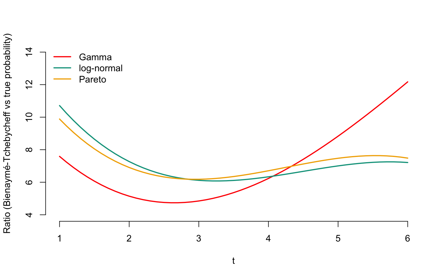
Figure 4.1: Evoluation of ratios between Bienaymé-Tchebycheff upper bound and the true probability

4.5 Insurance and Law of Large Numbers

4.5.1 Convergence in Probability

The law of large numbers provides a relevant justification for the calculation method of the pure premium associated with \(S\). To understand this, we need a concept of convergence for a sequence of random variables.

Definition 4.3 The sequence \(\{T_n,\hspace{2mm}n\in{\mathbb{N}}\}\) converges in probability to the random variable \(T\), denoted as \[ T_n\to_{\text{proba}}T, \] when \[ \Pr\big[|T_n-T|>\epsilon\big]\to 0\mbox{ as }n\to +\infty \] for any \(\epsilon>0\).

This expresses the fact that as \(n\) increases, the probability that \(T_n\) deviates from its limit \(T\) by more than \(\epsilon\) tends towards 0; \(T_n\) gets closer to its limit \(T\) as \(n\) gets larger.

4.5.2 Convergence of Average Claim Amount per Policy to the Pure Premium

4.5.2.1 Law of Large Numbers

Let’s assume that the insurer issues a large number of identical policies, and let \(S_i\), \(i=1,2,\ldots,n\), represent the total payout by the insurer related to policy number \(i\) during a reference period (usually a year).

Proposition 4.9 Let \(\mu\) and \(\sigma^2\) be the common mean and variance of the \(S_i\). Define \(\overline{S}^{(n)}\) as the average claim amount per policy, i.e. \[ \overline{S}^{(n)}=\frac{1}{n}\sum_{i=1}^nS_i. \] As long as the random variables \(S_i\) are independent, identically distributed, and have finite variance, the law of large numbers assures that \[ \overline{S}^{(n)}\to_{\text{proba}}\mu\mbox{ as }n\to +\infty. \]

Proof. Indeed, the inequality (4.7) guarantees that \[\begin{equation} \Pr\Big[\big|\overline{S}^{(n)}-\mu|>\epsilon\Big]\leq\frac{\mathbb{V}\Big[\overline{S}^{(n)}\Big]}{\epsilon^2}= \frac{\sigma^2}{n\epsilon^2}\to 0\mbox{ as }n\to +\infty.\tag{4.11} \end{equation}\]

We have thus established that the average claim amount per policy converges to the pure premium. By charging each policyholder an amount of \(\mu\), the company should have sufficient funds to compensate for the losses incurred, with no profit and no deficit.

4.5.2.2 Underlying Assumptions

It’s worth examining the assumptions underlying (4.11) cautiously, in order to identify situations where using mathematical expectation to calculate the pure premium might not be appropriate:

  1. Firstly, this result is asymptotic (as “\(n\) tends to infinity”). In practice, the portfolio size must be considerable for the law of large numbers to be applicable.
  2. Secondly, the random variables \(S_i\) are assumed to be independent. Insurance covering natural catastrophes like floods or earthquakes, which likely affect all risks in a specific geographical area, falls outside the scope of the law of large numbers.
  3. Lastly, the random variables \(S_i\) are assumed to be identically distributed. Risks grouped for insurance must be homogeneous, meaning they are of similar nature. There are several aspects of homogeneity:
  • Homogeneity in nature: Each risk must be categorized based on its nature. Risks such as “fire” and “liability” cannot be grouped together for statistical analysis. Within each category, further sub-classifications should correspond to similar risk characteristics. For instance, fire risks may be divided into simple risks and industrial risks. Liability risks could be categorized into tenant liability, family liability, etc.
  • Homogeneity in object: Risks must involve similar individuals or objects. In life insurance, individuals must be categorized by age, gender, and health status. In accident insurance, the profession of the individual should be taken into account (an actuary is a better risk than a construction painter).
  • Homogeneity in value: Risks should be grouped by their value. All risks don’t need to have the same significance, but there shouldn’t be a significant disparity in value among them.

If the risks are not sufficiently numerous, similar, and independent, the law of large numbers won’t be applicable, and risk pooling won’t be feasible. In such a situation, the insurer might consider reinsurance, which involves transferring a portion of the underwritten risks to another company.

Remark. It’s possible that for a given coverage, the portfolio of policies allows for risk pooling (satisfying the assumptions of the law of large numbers), but this might not hold true for another coverage. For example, consider an insurer covering fire damage for a large number of identical buildings located in the same city but not adjacent to each other. The principle of risk pooling will likely work well, with all three assumptions of the law of large numbers satisfied. However, these same buildings may not be independent risks for earthquake or flood coverage, necessitating the insurer to seek reinsurance.

4.5.2.3 Unit Premiums and Probabilities

We are now in a position to justify the interpretation of the probability of an event as the pure premium associated with a policy that pays 1if the event occurs. In this case, the insurer’s payout can be represented by the random variable \[ S=\mathbb{I}[E]=\left\{ \begin{array}{l} 1,\text{ if }E\text{ occurs},\\ 0,\text{ otherwise}. \end{array} \right. \] Clearly, \(S\sim\mathcal{B}er(\Pr[E])\), and the associated pure premium is \(\mathbb{E}\big[\mathbb{I}[E]\big]=\Pr[E]\).

4.5.3 Case of Flat Indemnity

4.5.3.1 At Most One Claim per Period

Let’s assume the insurer covers \(n\) individuals. In the event of a claim, the company is obligated to pay a flat amount \(s\). Each policy results in at most one claim. The random variable \(S_i\) representing the company’s reimbursement to individual \(i\) is given by \[\begin{equation} S_i=\left\{ \begin{array}{l} 0,\text{ with probability }1-q, \\ s,\text{ with probability }q. \end{array} \right.\tag{4.12} \end{equation}\] If the \(S_i\) are independent, then \[ \overline{S}^{(n)}\to_{\text{proba}}\mathbb{E}[S_1]=qs. \] The difference between \(\overline{S}^{(n)}\) and the pure premium \(qs\) is bounded using the Bienaymé-Chebyshev inequality by \[ \Pr\Big[|\overline{S}^{(n)}-qs|>\epsilon\Big]\leq\frac{1}{n\epsilon^2}s^2q(1-q). \]

4.5.3.2 Random Number of Claims per Period

If the policy can generate more than one claim per period, and the occurrence of any of these claims obligates the insurer to pay \(s\), the company’s expenditure is given by \(S_i=sN_i\), where \(N_i\) is the number of claims reported by policy \(i\).

In this case, \[ \overline{S}^{(n)}=s\overline{N}^{(n)}\text{ where }\overline{N}^{(n)}=\frac{1}{n}\sum_{i=1}^nN_i \text{ and }\overline{S}^{(n)}\to_{\text{proba}} s\mathbb{E}[N_1]. \] The difference between \(\overline{S}^{(n)}\) and the pure premium is controlled by \[ \Pr\Big[|\overline{S}^{(n)}-s\mathbb{E}[N_1]|>\epsilon\Big]\leq\frac{1}{n\epsilon^2}s^2\mathbb{V}[N_1]. \]

4.5.4 Case of Indemnity Compensation

4.5.4.1 Without Considering the Number of Claims

Now, suppose there’s a probability \(q\) that \(S_i>0\), and let \(Z_i\) be the amount of the claims when \(S_i>0\), i.e. \[\begin{equation} S_i=\left\{ \begin{array}{l} 0,\text{ with probability }1-q, \\ Z_i,\text{ with probability }q, \end{array} \right.\tag{4.13} \end{equation}\] where \(Z_1,Z_2,\ldots\) are positive, independent, and identically distributed random variables. In this case, the pure premium will be \(\mathbb{E}[S_i]=q\mathbb{E}[Z_i]=q\mu\).

We can represent \(S_i\) as \(J_iZ_i\) where \(J_i=\mathbb{I}[S_i>0]\). This time, the difference between \(\overline{S}^{(n)}\) and the pure premium \(q\mu\) is bounded using the Bienaymé-Chebyshev inequality by \[\begin{eqnarray*} \Pr\Big[|\overline{S}^{(n)}-q\mu|>\epsilon\Big]&\leq&\frac{1}{n\epsilon^2}\mathbb{V}[S_1]\\ &=&\frac{1}{n\epsilon^2}\big(q\sigma^2+\mu^2q(1-q)\big), \end{eqnarray*}\] where \(\sigma^2=\mathbb{V}[Z_1]\).

Remark. In some cases, it might be useful for the actuary to explicitly include the number of claims made by the insured. In this case, the model could be represented as \[ S_i=\sum_{k=1}^{N_i}C_{ik}. \] The pure premium would then be \[ \mathbb{E}[S_i]=\mathbb{E}[N_i]\mathbb{E}[C_{i1}]. \]

4.6 Characteristic Functions

4.6.1 Probability Generating Function

4.6.1.1 Definition

The probability generating function is a convenient tool for obtaining a series of valuable results for actuaries, although it lacks an intuitive interpretation. It is defined as follows.

Definition 4.4 The probability generating function of a random variable \(N\) taking values in \(\mathbb{N}\), denoted by \(\varphi_N\), is defined as \[ \varphi_N(z)=\mathbb{E}[z^N]=\sum_{j\in\mathbb{N}}\Pr[N=j]z^j, \quad 0\leq z\leq 1. \]

This function characterizes the probability distribution of \(N\). In fact, the successive derivatives of \(\varphi_N\) evaluated at \(z=0\) provide the probabilities \(\Pr[N=k]\) with a factor, i.e., \[\begin{eqnarray*} \Pr[N=0]&=&\varphi_N(0),\\ k!\Pr[N=k] &=& \left.\frac{d^k}{dz^k}\varphi_N(z)\right|_{z=0}, \quad k\geq 1. \end{eqnarray*}\] The successive derivatives of \(\varphi_N\) evaluated at \(z=1\) provide the factorial moments, namely \[\begin{eqnarray*} \left.\frac{d}{dz}\varphi_N(z)\right|_{z=1} & = & \mathbb{E}[N],\\ \left.\frac{d^k}{dz^k}\varphi_N(z)\right|_{z=1} &=& \mathbb{E}[N(N-1)\ldots(N-k+1)], \quad k\geq 1. \end{eqnarray*}\] Note that, obviously, \(\varphi_N(1)=1\).

The probability generating functions associated with the common discrete probability distributions are listed in Table 4.3.

Table 4.3: Probability Generating Function of Common Discrete Distributions
Probability Law Probability Generating Function
\(\mathcal{DU}ni(n)\) \(\frac{1}{n+1}\frac{t^{n+1}-1}{t - 1}\)
\(\mathcal{B}er(q)\) \((1-q + q t)\)
\(\mathcal{B}in(m,q)\) \((1-q +qt)^m\)
\(\mathcal{G}eo(q)\) \(\frac{q}{1-(1-q)t}\)
\(\mathcal{NB}in(\alpha,q)\) \(\left( \frac{q}{1-(1-q)t} \right) ^\alpha\)
\(\mathcal{P}oi(\lambda)\) \(\exp( \lambda (t -1))\)

4.6.1.2 Probability Generating Function and Convolution

The main advantage of the probability generating function lies in its easy handling of convolutions. If we want to find the probability generating function of a sum of independent counting variables, we only need to multiply the probability generating functions of each term, as shown by the following result.

Proposition 4.10 The probability generating function of \(N_\bullet=\sum_{i=1}^nN_i\), where the \(N_i\) are independent, is given by the product of the generating functions \(\varphi_{N_i}\) of each term.

Proof. We just need to write \[\begin{eqnarray*} \varphi_{N_\bullet}(z) & = & \mathbb{E}\left[z^{\sum_{i=1}^nN_i}\right]=\mathbb{E}\left[\prod_{i=1}^n z^{N_i}\right] \\ & = & \prod_{i=1}^n\mathbb{E}[z^{N_i}]=\prod_{i=1}^n\varphi_{N_i}(z),\quad z\in[0,1]. \end{eqnarray*}\]

In particular, if \(N_1,\ldots,N_n\) are independent and identically distributed, we have \[ \varphi_{N_\bullet}(z)=\{\varphi_{N_1}(z)\}^n. \]

Example 4.13 (Convolution of Binomial Distributions with Same Parameter) Let’s consider two independent random variables \(N_1\) and \(N_2\) with distributions \(\mathcal{B}in(m_1,q)\) and \(\mathcal{B}in(m_2,q)\) respectively. The probability generating function of the sum \(N_1+N_2\) is given by \[ \varphi_{N_1+N_2}(z)=\varphi_{N_1}(z)\varphi_{N_2}(z)=\big(1+q(z-1)\big)^{m_1+m_2}, \] which shows that \(N_1+N_2\sim\mathcal{B}in(m_1+m_2,q)\). Therefore, the Bernoulli distribution provides the foundation for the binomial family, as any random variable \(N\) with a \(\mathcal{B}in(m,q)\) distribution can be represented as \[ N=\sum_{i=1}^mN_i, \] where the \(N_i\) are independent and follow a \(\mathcal{B}er(q)\) distribution.

Example 4.14 (Convolution of Poisson Distributions) Let \(N_1,N_2,\ldots,N_n\) be independent random variables with Poisson distributions and respective parameters \(\lambda_1,\lambda_2,\ldots,\lambda_n\). Then \(N=\sum_{i=1}^nN_i\) follows a Poisson distribution with parameter \(\sum_{i=1}^n\lambda_i\). The probability generating function of \(N\) is the product of the probability generating functions of the \(N_i\): \[ \varphi_N(z)=\prod_{i=1}^n\exp(\lambda_i(z-1)) =\exp\left((z-1)\sum_{i=1}^n\lambda_i\right), \] which makes \(N\) a random variable with a Poisson distribution with parameter \(\sum_{i=1}^n\lambda_i\).

4.6.2 Laplace Transform

4.6.2.1 Definition

Similar to the probability generating function, the Laplace transform does not have an intuitive interpretation. Again, it is a useful tool for obtaining results in risk theory. This function characterizes the distribution of \(X\) and is defined as follows.

Definition 4.5 The Laplace transform of a random variable \(X\), denoted by \(L_X\), is given by \[ L_X(t)=\mathbb{E}[\exp(-tX)],\quad t\geq 0. \]

Laplace transform is often used for non-negative random variables. This ensures its existence and makes it a convenient tool for solving many problems in applied probability.

The moments of \(X\) can be easily obtained by differentiating \(L_X\) and evaluating the derivatives at 0. Specifically, \[ \mathbb{E}[X^k]=(-1)^k\left.\frac{d^k}{dt^k}L_{X}(t)\right|_{t=0}, \quad k\in \mathbb{N}. \]

Table 4.4 presents the Laplace transforms associated with common continuous probability distributions.

Table 4.4: Laplace Transforms of Common Continuous Probability Distributions.
Probability Law Laplace transform \(L_X(t)\)
\(\mathcal{U}ni(a,b)\) \(\frac{\exp(-at)-\exp(-bt)}{(b-a)t}\)
\(\mathcal{B}et(\alpha,\beta)\) No explicit form
\(\mathcal{N}or(\mu,\sigma^2)\) \(\exp(-\mu t+\frac{1}{2}\sigma^2t^2)\)
\(\mathcal{E}xp(\theta)\) \(\left(1+\frac{t}{\theta}\right)^{-1}\)
\(\mathcal{G}am(\alpha,\tau)\) \(\left(1+\frac{t}{\tau}\right)^{-\alpha}\)
\(\mathcal{LN}or(\mu,\sigma^2)\) No explicit form
\(\mathcal{P}ar(\alpha,\theta)\) No explicit form

4.6.2.2 Bernstein’s Theorem

Bernstein’s theorem provides a necessary and sufficient condition for a function to be the Laplace transform of a probability distribution. To do this, recall that a function \(g:{\mathbb{R}}^+\to{\mathbb{R}}\) is completely monotone if its derivatives \(g^{(k)}\) of all orders satisfy \[ (-1)^kg^{(k)}(t)\geq 0\mbox{ for all }t>0. \]

Proposition 4.11 (Bernstein's Theorem) A function \(g\) is the Laplace transform of a positive random variable if and only if it is completely monotone and satisfies \(g(0)=1\).

4.6.2.3 Laplace Transform and Convolution

The Laplace transform plays an important role in the analysis of convolutions, as shown by the following result.

Proposition 4.12 Given non-negative and independent random variables \(X_1,X_2,\ldots,X_n\), denoting their sum as \(S=\sum_{i=1}^nX_i\), the Laplace transform \(L_S\) of \(S\) is given by the product of the Laplace transforms \(L_{X_i}\) of each term.

Proof. We can write \[\begin{eqnarray*} L_S(t)&=&\mathbb{E}\left[\exp\left(-t\sum_{i=1}^nX_i\right)\right] \\ &=&\mathbb{E}\left[\prod_{i=1}^n\exp\left(-tX_i\right)\right] \\ &=&\prod_{i=1}^n L_{X_i}(t),\quad t\geq 0. \end{eqnarray*}\]

Thus, under the assumption of independence, we can easily obtain the Laplace transform of the sum of the \(X_i\), while obtaining the corresponding cumulative distribution function is often very difficult.

Example 4.15 (Convolution of Gamma Distributions) The Laplace transform expression of the \(\mathcal{G}am(\alpha,\tau)\) distribution given in Table 4.4 reveals a fundamental property of the gamma distribution: its stability under convolution. Indeed, if \(X_1\) and \(X_2\) are independent random variables with distributions \(\mathcal{G}am(\alpha_1,\tau)\) and \(\mathcal{G}am(\alpha_2,\tau)\) respectively, then \(X_1+X_2\) follows a \(\mathcal{G}am(\alpha_1+\alpha_2,\tau)\) distribution. To see this, notice that the Laplace transform of \(X_1+X_2\) is \[ \left(1+\frac{t}{\tau}\right)^{-\alpha_1} \left(1+\frac{t}{\tau}\right)^{-\alpha_2} =\left(1+\frac{t}{\tau}\right)^{-\alpha_1-\alpha_2} \] which indeed corresponds to the \(\mathcal{G}am(\alpha_1+\alpha_2,\tau)\) distribution.

4.6.2.4 Laplace Transform of Compound Distributions

The following property will be useful, especially in Chapter 9, to approximate compound distributions corresponding to mixed distribution variables (??).

Proposition 4.13 The Laplace transform of \(S\) defined in (??), i.e. \(S=\sum_{i=1}^NX_i\) with \(X_i\), \(i=1,2,\ldots\), independent and identically distributed, and independent of \(N\), is given for \(t>0\) by \(L_S(t)=\varphi_N(L_{X_1}(t))\).

Proof. We can write \[\begin{eqnarray*} L_S(t) & = & \mathbb{E}\left[\exp\left(-t\sum_{i=1}^NX_i\right)\right] \\ & = & \sum_{k=0}^{+\infty}\Pr[N=k]\mathbb{E}\left[\exp\left(-t\sum_{i=1}^kX_i \right)\right] \\ & = & \sum_{k=0}^{+\infty}\Pr[N=k]\{L_{X_1}(t)\}^k = \varphi_N(L_{X_1}(t)). \end{eqnarray*}\]

Example 4.16 As \(\varphi_{N}(z)=\exp\{\lambda(z-1)\}\) when \(N\sim\mathcal{P}oi(\lambda)\), the Laplace transform of \(S\sim\mathcal{CP}oi(\lambda,F_X)\) is \[ L_S(t)=\exp\{\lambda(L_X(t)-1)\},\quad t\in {\mathbb{R}}^+. \]

4.6.2.5 Stability of Compound Poisson Distribution through Convolution

Laplace transforms are quite useful for obtaining results involving convolutions, like the following property.

Proposition 4.14 Consider independent random variables \(S_1\sim\mathcal{CP}oi(\lambda_1,F_1)\), , \(S_n\sim\mathcal{CP}oi(\lambda_n,F_n)\). Then \[ S=\sum_{j=1}^nS_j\sim\mathcal{CP}oi(\lambda_\bullet,F_\bullet), \] where \[ \lambda_\bullet=\sum_{j=1}^n\lambda_j\text{ and }F_\bullet(x)=\frac{1}{\lambda_\bullet} \sum_{j=1}^n\lambda_jF_j(x),\quad x\in\mathbb{R}. \]

Proof. It is enough to write \[ L_S(t)=\prod_{j=1}^nL_{S_j}(t)=\prod_{j=1}^n\exp\{\lambda_j(L_j(t)-1)\}, \] where \(L_j\) is the Laplace transform of the distribution corresponding to the cumulative distribution function \(F_j\). The result is then obtained by noticing that \[ L_s(t)=\exp\{\lambda_\bullet(L_\bullet(t)-1)\}, \] where the Laplace transform \[ L_\bullet(t)=\frac{1}{\lambda_\bullet}\sum_{j=1}^n\lambda_jL_j(t) \] corresponds to the cumulative distribution function \(F_\bullet\).

4.6.2.6 The Case of Infinite Variance Risks

We saw in Property 4.9 that the law of large numbers guarantees (under certain assumptions) the convergence of the average claim amount to the pure premium. However, the reasoning based on (??) assumes that the \(S_i\) have finite variance. The result still holds if the \(S_i\) have infinite variance (which is sometimes the case when the actuary deals with very large claim amounts, invoking the Pareto distribution).

Proposition 4.15 Let \(S_1,S_2,\ldots,S_n\) be non-negative, independent, and identically distributed random variables with finite mean. Then \(\overline{S}^{(n)}\to_{\text{prob}}\mu\) as \(n\to +\infty\).

Proof. Let \(L_S\) be the common Laplace transform of the \(S_i\). The Laplace transform of the sum \(S_1+S_2+\ldots+S_n\) is \(L_S^n\), and that of \(\overline{S}^{(n)}\) is \[ L_{\overline{S}^{(n)}}(t)=\left\{L_S\left(\frac{t}{n}\right)\right\}^n. \] Now, a limited Taylor expansion (to the first order) gives \[ L_S(t)=1-\mu t+o(t), \] where \(o(t)\) is such that \[ \lim_{t\to 0}\frac{o(t)}{t}=0, \] i.e., a function that tends to 0 faster than the identity function (\(o(t)\) is negligible for small values of \(t\)). Therefore, as \(n\to +\infty\) \[\begin{eqnarray*} \lim_{n\to +\infty}L_{\overline{S}^{(n)}}(t)&=&\lim_{n\to +\infty}\left\{L_S\left(\frac{t}{n}\right)\right\}^n\\ &=&\lim_{n\to +\infty}\left\{1-\frac{\mu t}{n}\right\}^n=\exp(-t\mu). \end{eqnarray*}\] Since \(\exp(-t\mu)\) is the Laplace transform associated with the constant \(\mu\), we indeed recover the convergence of \(\overline{S}^{(n)}\) to \(\mu\).

Thus, coverage of risks with infinite variance remains possible. However, intuitively, we can sense that it would be a risky endeavor—it deals with risks for which the spread around the pure premium is infinite!

4.6.3 Moment Generating Function

4.6.3.1 Definition

The moment generating function complements the actuary’s toolkit. It naturally appears in ruin theory and allows for classifying probability distributions according to their associated risks. Unlike the Laplace transform, it is not always defined for non-negative random variables.

Definition 4.6 Given a random variable \(X\), its moment generating function \(M_X\) is defined as \[ M_X(t)=\mathbb{E}[\exp(tX)],\quad t\geq 0. \]

We can see that the difference between the Laplace transform and the moment generating function is essentially formal (\(-t\) is replaced by \(t\)). In actuarial science, it is customary to distinguish between these two tools.

4.6.3.2 Log-Normal Distribution

The moments of the log-normal distribution can be easily obtained from the moment generating function of the normal distribution, as shown in the following example.

Example 4.17 (Moments of the Log-Normal Distribution) When \(X\sim\mathcal{LN}or(\mu,\sigma^2)\), \(X\) has the same distribution as \(\exp(Y)\) where \(Y\sim\mathcal{N}or(\mu,\sigma^2)\). Therefore, \[\begin{eqnarray*} \mathbb{E}[X]=\mathbb{E}[\exp(Y)] & = & M_Y(1)=\exp(\mu+\sigma^2/2), \end{eqnarray*}\] and \[ \mathbb{E}[X^2]=M_Y(2)=\mathbb{E}[\exp(2Y)]=\exp(2\mu+2\sigma^2), \] from which we deduce \[\begin{eqnarray*} \mathbb{V}[X]&=&\exp(2\mu+2\sigma^2)-\exp(2\mu+\sigma^2)\\ &=&\exp(2\mu)\exp(\sigma^2)(\exp(\sigma^2)-1). \end{eqnarray*}\] Thus, the two parameters \(\mu\) and \(\sigma^2\) influence the variability of \(X\).

However, an exponential decay of the tail does not necessarily guarantee the finiteness of the moment generating function. The example of the log-normal distribution illustrates this point. All the moments associated with this distribution exist and are finite. Specifically, if \(X\sim\mathcal{LN}or(\mu,\sigma^2)\), then, generalizing Example 4.17: \[ \mathbb{E}[X^k]=\exp(k\mu+\frac{1}{2}k^2\sigma^2),\quad k=1,2,\ldots \] However, the moment generating function \(M_X(t)\) is always infinite, regardless of the value of \(t\). As a result, the Pareto distribution \(\mathcal{P}ar(\alpha,\theta)\) (for which moments of order \(k>\alpha\) are infinite) does not have a moment generating function.

4.6.3.3 Cramér’s Distribution

In addition to its use in certain mathematical developments, the moment generating function is a convenient tool for assessing the level of risk associated with a distribution used to model the cost of claims. Unlike the Laplace transform, the moment generating function is not necessarily finite. Distributions for which \(M_X\) is constantly infinite indicate a high level of risk for the insurer. The Log-Normal and Pareto distributions fall into this category.

On the contrary, Cramér’s distributions are those for which the moment generating function is finite for at least one positive value of its argument. Such distributions reflect a low or moderate degree of risk for the insurer.

Definition 4.7 The random variable \(X\) has a Cramér distribution if there exists \(h>0\) such that \(M_X(t)\) exists and is finite for \(t<h\).

We obtain by expanding the exponential in a Taylor series: \[ M_X(t)=1+\sum_{k=1}^{+\infty}\frac{t^k}{k!}\mathbb{E}[X^k]\text{ for }t<h. \]

Table 4.5 summarizes the moment generating functions of common continuous probability distributions.

Table 4.5: Moment generating functions of common continuous probability distributions.
Probability Law Moment Generating Function \(M_X(t)\)
\(\mathcal{U}ni(a,b)\) \(\frac{\exp(bt)-\exp(at)}{(b-a)t}\)
\(\mathcal{B}et(\alpha,\beta)\) no explicit form
\(\mathcal{N}or(\mu,\sigma^2)\) \(\exp(\mu t + \frac{1}{2}\sigma^2t^2)\)
\(\mathcal{E}xp(\theta)\) \(\left(1-\frac{t}{\theta}\right)^{-1}\) if \(t<\theta\)
\(\mathcal{G}am(\lambda, \alpha)\) \(\left(1-\frac{t}{\tau}\right)^{-\alpha}\) if \(t<\tau\)

4.6.3.4 Moment Generating Function and Convolution

Similar to the Laplace transform, the primary interest of the moment generating function lies in the study of sums of random variables. Indeed, the sum of independent random variables amounts to taking the product of the moment generating functions.

Given non-negative independent random variables \(X_1,X_2,\ldots,X_n\), and denoting their sum as \(S=\sum_{i=1}^nX_i\), the moment generating function \(M_S\) of \(S\) is given by the product of the moment generating functions \(M_{X_i}\) of each term.

Proof. It suffices to write \[\begin{eqnarray*} M_S(t)&=&\mathbb{E}\left[\exp\left(t\sum_{i=1}^nX_i\right)\right]\\ &=&\mathbb{E}\left[\prod_{i=1}^n\exp(tX_i)\right]\\ &=&\prod_{i=1}^nM_{X_i}(t). \end{eqnarray*}\]

Example 4.18 (Convolution of Normal Distributions) If \(X\sim\mathcal{N}or(\mu,\sigma^2)\), \[ M_X(t)=\exp(\mu t+\frac{1}{2}t^2\sigma^2). \] This allows us to assert that given independent random variables \(X_i\sim\mathcal{N}or(\mu_i,\sigma_i^2)\), any linear combination \(T=\sum_{i=1}^n\alpha_iX_i\) is also normally distributed. Indeed, the moment generating function of \(T\) is given by \[ \prod_{i=1}^n\mathbb{E}[\exp(\alpha_itX_i)]=\exp\left(\sum_{i=1}^n\alpha_i\mu_i+\frac{t^2}{2}\sum_{i=1}^n\alpha_i^2\sigma_i^2\right), \] which implies that \[ \sum_{i=1}^n\alpha_iX_i\sim\mathcal{N}or\left(\sum_{i=1}^n\alpha_i\mu_i,\sum_{i=1}^n\alpha_i^2\sigma_i^2\right). \]

4.6.3.5 Chernoff Bound

This very useful bound holds for Cramér’s distributions.

Proposition 4.16 Let \(X\) be a random variable with a finite moment generating function, and denote \[ \Psi(t)=\ln M_X(t). \] We have \[ \overline{F}_X(x)\leq\exp(-h(x))\text{ where }h(x)=\sup_{t\geq 0}\{tx-\Psi(t)\}. \]

Proof. The Markov inequality stated in Property ?? gives \[\begin{eqnarray*} \overline{F}_X(x)&=&\Pr[\exp(tX)>\exp(tx)]\\ &\leq&\frac{M_X(t)}{\exp(tx)}=\exp(-(tx-\Psi(t))). \end{eqnarray*}\] Since the above reasoning applies for any \(t>0\), we deduce the announced result from the existence of a moment generating function.

A random variable with a moment generating function must therefore necessarily have a tail function that exponentially decreases to 0.

4.6.4 Hazard Rate

4.6.4.1 Definition

An interesting quantity is the hazard rate (also known as the instantaneous death rate in life insurance), defined as follows.

Definition 4.8 Let \(X\) be a positive random variable with a probability density function \(f_X\). The hazard rate associated with \(X\), denoted as \(r_X\), is given by \[\begin{equation} r_X(x)=-\frac{d}{dx}\ln\overline{F}(x)=\frac{f_X(x)}{\overline{F}_X(x)},\hspace{2mm} x\in {\mathbb{R}}^+.\tag{4.14} \end{equation}\]

4.6.4.2 Interpretation

To better understand the meaning of the hazard rate, it is useful to refer to the following representation of \(r_X\).

Proposition 4.17 The hazard rate can be obtained through the following limit: \[ r_X(x)=\lim_{\Delta x\to 0}\frac{\Pr[x<X\leq x+\Delta x|X>x]} {\Delta x}. \]

Proof. Indeed, \[\begin{eqnarray*} \Pr[x<X\leq x+\Delta x|X>x] & = & \frac{\Pr[x<X\leq x+\Delta x]}{\Pr[X>x]} \\ & = & \frac{\Pr[X>x]-\Pr[X>x+\Delta x]}{\Pr[X>x]}, \end{eqnarray*}\] thus \[\begin{eqnarray*} & & \lim_{\Delta x\to 0}\frac{\Pr[x<X\leq x+\Delta x|X>x]} {\Delta x} \\ & = & \frac{1}{\Pr[X>x]}\lim_{\Delta x\to 0}\frac{\Pr[X>x]-\Pr[X>x+\Delta x]} {\Delta x} \\ & = & -\frac{1}{\Pr[X>x]}\frac{d}{dx}\Pr[X>x] =r_X(x). \end{eqnarray*}\]

In other words, \(r_X(x)\Delta x\) can be interpreted as the probability that the claim amount is approximately equal to \(x\) given that it is at least \(x\). Formally, the hazard rate of a risk \(X\) allows us to approximate the “probability” that \(X\) is equal to \(x\), given that \(X\) exceeds \(x\), i.e. \[ r_X(x)\Delta x\approx \Pr[x<X\leq x+\Delta x|X>x]. \]

Remark. It is interesting to compare this interpretation with the one held by the density function. We have seen in the previous chapter that the density function \(f_X\) of a risk \(X\) evaluated at \(x\) can be interpreted as the “probability” that \(X\) is “equal” to \(x\), since \[ f_X(x)=\lim_{\Delta x\to 0}\frac{\Pr[x<X\leq x+\Delta x]}{\Delta x}, \] so that the approximation \[ f_X(x)\Delta x\approx \Pr[x<X\leq x+\Delta x] \] is valid for sufficiently small \(\Delta x\).

4.6.4.3 Connection with the Tail Function

The following result shows that it is possible to express the tail function of \(x\) in terms of the hazard rate \(r_X\).

Proposition 4.18 The tail function of a positive random variable \(X\) is expressed as follows in terms of the associated hazard rate \(r_X\): \[\begin{equation} \overline{F}(x)=\exp\left(-\int_{\xi=0}^xr_X(\xi)d\xi\right), \hspace{2mm}x\geq 0.\tag{4.15} \end{equation}\]

Proof. It is sufficient to solve the differential equation (4.14) with the initial condition \(\overline{F}(0)=1\).

Property 4.18 shows that the hazard rate \(r_X\) characterizes the probability distribution of \(X\).

4.6.5 Stop-Loss Premiums

4.6.5.1 Definition

A stop-loss reinsurance treaty involves having the reinsurer take over the part of the total claim amount \(S\) that exceeds a certain amount \(d\). The reinsured portion, denoted as \(S^R\), is thus defined by \[ S^R=(S-d)_+=\left\{ \begin{array} {l} 0, \mbox{ if } S\leq d,\\ S-d, \mbox{ if } S>d. \end{array} \right. \] Note that this risk transfer between the insurer and the reinsurer is similar to the mandatory deductible clause imposed on insured parties by an insurance company, a clause that we examined in detail in Section 3.15.2.

The pure premium that the cedent must pay to the reinsurer for such a contract, called the stop-loss premium, is given by \[ \mathbb{E}[S^R]=\mathbb{E}[(S-d)_+]. \] This leads to the following definition.

Definition 4.9 Given a risk \(X\), the stop-loss premium for a retention \(t\geq 0\) is defined as \[ \pi_X(t) = \mathbb{E}[(X-t)_+] . \] The function \(\pi_X\) is also called the stop-loss transform of the random variable \(X\).

Remark. Even though formally there is no distinction between the stop-loss premium \(\mathbb{E}[(X-t)_+]\) and the price of a call option on an asset whose value at the exercise time is \(X\) and \(t\) denotes the exercise price, they are two quite different mathematical entities.

Indeed, the stop-loss premium is calculated using the physical or historical probability distribution, while in the case of the call option, a change of measure is applied beforehand to switch to the risk-neutral probability distribution (which avoids arbitrage opportunities).

Apart from the fact that insurance markets are incomplete, invalidating many results from classical financial theory, the actuary works with the historical probability measure, while the financier switches to the risk-neutral measure.

4.6.5.2 Properties

Integration by parts yields the following result quite easily.

Proposition 4.19 The stop-loss transform can be expressed as follows using the tail function: \[\begin{equation} \pi_X(t)=\int_{x=t}^{+\infty}\overline{F}_X(x)dx.\tag{4.16} \end{equation}\]

Representation (4.16) also allows us to derive the following characteristics of the stop-loss transform \(\pi_X\).

Proposition 4.20 Assuming \(\mathbb{E}[X]<+\infty\). The stop-loss transform \(\pi_X\) has the following properties:

  1. It is decreasing and convex.
  2. \(\lim_{t\to +\infty}\pi_X(t)=0\) and \(\lim_{t\to -\infty}\{\pi_X(t)+t\}=\mathbb{E}[X]\).

Proof.

  1. is immediately deduced from the representation (4.16). As for (2), the first limit is obtained from (4.16), while the second comes from \[ \lim_{t\to -\infty}\{\pi_X(t)+t\}=\lim_{t\to -\infty}\mathbb{E}[\max\{X,t\}]=\mathbb{E}[X]. \]

The following property is also quite interesting. It states that a function satisfying conditions (1)-(2) in Property 4.20 is the stop-loss transform associated with a risk \(X\).

Proposition 4.21 If the function \(g\) satisfies (1)-(2) in Property 4.20, there exists a risk \(X\) such that \(g=\pi_X\). The cumulative distribution function of \(X\) is given by \[ F_X(t)=1+g_+'(t), \] where \(g_+'\) is the right derivative of \(g\).

Proof. If \(g\) is convex, then the right derivative \(g_+'\) exists and is non-decreasing and continuous from the right. Additionally, \[ \lim_{t\to +\infty}g(t)=0\Rightarrow \lim_{t\to+\infty}g_+'(t)=0 \] and \(\lim_{t\to -\infty}\{g(t)+t\}\) can only exist if \(\lim_{t\to -\infty}g_+'(t)=-1\). Thus, \(1+g_+'\) is a distribution function, denoted as \(F_X\). Taking \(X=F_X^{-1}(U)\) concludes the proof.

Remark. Property 4.21 also teaches us that the stop-loss transform \(\pi_X\) characterizes the probability distribution of \(X\).

4.6.5.3 Average Excess of Loss

Another interesting quantity in the analysis of claim distributions, quite similar to the stop-loss premium, is the average excess of loss (also known as remaining lifetime in life insurance), defined as follows.

Definition 4.10 Given a risk \(X\), the average excess of loss \(e_X\) is defined as \[\begin{eqnarray*} e_X(x) & = & \mathbb{E}[X-x|X>x] \\ & = & \frac{\int_{\xi=x}^{+\infty}(\xi-x)dF_X(\xi)}{\overline{F}_X(x)}, \hspace{2mm}x\geq 0. \end{eqnarray*}\]

It represents the average claim amount when a mandatory deductible of amount \(x\) is applied by the company. A distribution for which \(e_X\) only slowly tends to 0 is less favorable for the insurer compared to another distribution where the convergence to 0 is rapid.

The average excess of loss for common continuous distributions is presented in Table 4.6 (including their asymptotic behavior as \(x\to +\infty\)). Starting from (4.16), it is straightforward to observe that \[ \pi_X(t)=e_X(t)\overline{F}_X(t), \] so that the stop-loss premiums associated with common probability distributions can be derived easily from Table 4.6.

Table 4.6: Average Excess of Loss for common continuous probability distributions.
Probability law Average Excess of Loss Asymptotic Equivalent \((x\to +\infty)\)
\(\mathcal{E}xp(\theta)\) \(\frac{1}{\theta}\)
\(\mathcal{G}am(\alpha,\tau)\) \(\frac{\alpha}{\tau}\frac{1-\Gamma(\alpha+1,\tau x)}{1-\Gamma(\alpha,\tau x)}-x\) \(\frac{1}{\tau}\)
\(\mathcal{LN}or(\mu,\sigma^2)\) \(\exp(\mu+\frac{\sigma^2}{2})\frac{\overline{\Phi}\left(\frac{\ln(x)-\mu-\sigma^2}{\sigma}\right)}{\overline{\Phi}\left(\frac{\ln(x)-\mu}{\sigma}\right)}-x\) \(\sigma^2\frac{x}{\ln x}\)
\(\mathcal{P}ar(\alpha,\theta)\) with \(\alpha>1\) \(\frac{\theta+x}{\alpha-1}\)

4.7 Heterogeneity and Mixtures

4.8 Context

So far, we have assumed that the risks in the portfolio are independent and identically distributed. In most insurances sold to the general public, the dependence between insured risks is not a major issue. In automobile liability insurance, family liability insurance, or theft insurance, it is usually negligible. In fire insurance, it can be easily managed through proper underwriting practices or an appropriate reinsurance program. However, in some cases, the actuary must carefully examine the consequences of dependence; examples include the “earthquake” or “flood” component of fire insurance. The assumption of identical distribution, however, is much less clear. It is clear that certain characteristics of risks influence the probability of a claim occurring or the extent of its consequences.

One of the key features of insurance is that not all individuals are equal in the face of risk: some have a propensity to cause much higher or more frequent claims than others. When these insured parties are mixed in the insurer’s portfolio, it results in some heterogeneity: individuals with a low level of risk coexist with others whose risk level is higher. The insurer can partially address this problem by partitioning the portfolio into more homogeneous risk classes. As we will see later, this is achieved by using observable characteristics of insured parties that significantly influence risk. Even if the portfolio is divided into sub-classes, they often remain very heterogeneous. This heterogeneity of risks covered by the insurer is captured by the mixture models we study in this section.

4.8.1 A Simple Example…

4.8.1.1 A Portfolio with Two Types of Risks

Let’s revisit Example ?? and assume that the risk of loss or theft of luggage varies depending on the traveler’s destination. For countries in group A, let’s say the insurer has to pay the fixed indemnity of 250in 10% of cases, on average, while for countries in group B, the fixed indemnity will be paid in 20% of cases. Thus, for travelers to countries in group A, the insurer’s expense is represented by the random variable \[ S_A=\left\{ \begin{array}{l} 0,\text{ with probability }0.9,\\ 250\text{Euros},\text{ with probability }0.1 \end{array} \right. \] while for a traveler to countries in group B, the expense becomes \[ S_B=\left\{ \begin{array}{l} 0,\text{ with probability }0.8,\\ 250\text{Euros},\text{ with probability }0.2. \end{array} \right. \]

4.8.1.2 Pure Premiums

The insurer should therefore charge a pure premium of \(\mathbb{E}[S_A]=25\text{Euros}\) for a traveler departing to a country in group A, compared to \(\mathbb{E}[S_B]=50\text{Euros}\) for another traveler heading to a country in group B. Suppose that 50% of trips are to countries in group A, and 50% to countries in group B. In the portfolio, 50% of insured parties who incur expenses according to the distribution of \(S_A\) coexist with the other half who incur expenses according to the distribution of \(S_B\). This portfolio is therefore heterogeneous, mixing two types of risks.

4.8.1.3 Total Pure Premium Income

The total premium income of the company for this portfolio is \[ n_A\mathbb{E}[S_A]+n_B\mathbb{E}[S_B]=75 n_A, \] where \(n_A\) represents the number of policies covering travelers to countries in group A, and \(n_B=n_A\) represents the number of policies covering travelers to countries in group B.

4.8.1.4 Associated Homogeneous Portfolio

In terms of pure premiums, there is no difference between this portfolio and a homogeneous portfolio in which the claim amounts for each policy would follow the distribution \[ S_{AB}=\left\{ \begin{array}{l} 0,\text{ with probability }0.85,\\ 250\text{Euros},\text{ with probability }0.15. \end{array} \right. \] Indeed, the total pure premium income for this homogeneous portfolio is \[ (n_A+n_B)37.5=75n_A. \] Considering the homogeneous portfolio is equivalent to neglecting to differentiate insured parties based on their destination, and thus on the risk they represent(We emphasize that there is no single correct practice. The actuary decides on the model based on the level of solidarity they want to induce in the portfolio. Their goal is not to automatically choose the model that best fits reality. Assuming that the \(S_i\) are independent and identically distributed when they are not amounts to inducing the maximum level of solidarity in the portfolio, which is not necessarily a bad thing). If we acknowledge the heterogeneity of the portfolio, we charge 25or 50based on the destination, while erasing this difference implies applying a uniform premium of 37.5to all insured parties in the portfolio.

4.8.1.5 Consequences of Portfolio Heterogeneity

This simple example introduces several fundamental concepts:

  1. When a uniform premium is charged to insured parties in a heterogeneous portfolio, a certain level of solidarity emerges. Indeed, the 37.5premium paid by an insured traveler to a country in group A can be broken down into a sum of 25, which is the price of their risk, and an additional 12.5, which will artificially lower the premium for travelers to countries in group B. The 25is paid due to risk pooling: it will be used to compensate claims affecting insured parties with the same profile (i.e., traveling to a country in group A). On the other hand, the 12.5reflects the solidarity that the insurer has introduced at the portfolio level by standardizing the premium amount.

  2. When a uniform premium is charged to insured parties in a heterogeneous portfolio, the induced solidarity makes the insurer’s results depend on the portfolio’s structure. For instance, imagine that insured parties traveling to countries in group A are well aware of their risk, realize they are overcharged, and decide not to purchase coverage anymore, deeming the product too expensive. The insurer would then only have insured parties whose destination is a country in group B in the portfolio. Its total pure premium income would amount to \(n_B37.5\text{Euros}\) and would not be sufficient to cover an expected loss of \(n_B50\text{Euros}\). Therefore, the collective premium of 37.5depends on the composition of the portfolio (here, the fact that 50% of trips are to countries in group A). Thus, the pricing is accurate only if the portfolio composition remains the same.

  3. The insurer can hardly maintain a uniform premium in a market where competitors differentiate risks and apply a balanced premium within each defined risk class. In our example, let’s assume that Company \(C_1\), the sole company on the market, charges 37.5to each insured party. A new company \(C_2\) enters the market and differentiates the premium amounts based on the destination country. The insured parties traveling to countries in group A should all switch from \(C_1\) to \(C_2\). The results of \(C_2\) will be balanced, but those of \(C_1\) will deteriorate rapidly, as the insured parties traveling to countries in group A will no longer be there to subsidize the discount granted to insured parties traveling to countries in group B. Company \(C_1\) will have no choice but to raise its uniform premium to 50(if it manages to overcome the loss of \(n_B 12.5\text{Euros}\) it will suffer in the first year when insured parties departing to countries in group A leave). Thus, the market, i.e., Companies \(C_1\) and \(C_2\), will acknowledge the risk difference based on the destination either explicitly (like \(C_2\), which offers a differentiated premium) or implicitly (like \(C_1\), whose pricing structure is such that it only targets a segment of the market).

However, it’s worth mentioning that reality is more subtle. Market players differentiate themselves not only by the premiums they charge but also by the services and extent of coverage they offer, by the target audience they address, and so on. Moreover, insured parties will only decide to switch their insurer if the premium reduction they obtain is substantial enough to justify the effort. The choice of the insurer can also be guided by ideological considerations, as is the case with mutuals.

4.8.1.6 Connection with Mixture Models

The random variable \(S\) representing the claim costs generated by a policy in the portfolio that mixes two types of risks can also be modeled as a mixture of two Bernoulli distributions (scaled by 250). That is, conditional on \(Q=q\), \(S\sim 250\mathcal{B}er(q)\) and \[ Q=\left\{ \begin{array}{l} 0.1,\text{ with probability }\frac{1}{2},\\ 0.2,\text{ with probability }\frac{1}{2}. \end{array} \right. \] Hence, mixture models provide an appropriate tool to handle the heterogeneity of insurance portfolios.

In general, we account for heterogeneity by introducing a random effect \(\Theta\) representing the unknown risk level of the insured party. This results in a mixture model, defined as follows.

Definition 4.11 Suppose that conditional on \(\{\Theta=\theta\}\), the distribution of the random variable \(X\) is described by the cumulative distribution function \(F(\cdot|\theta)\), i.e. \[ \Pr[X\leq x|\Theta=\theta]=F(x|\theta),\hspace{2mm}x\in{\mathbb{R}}. \] If \(\Theta\) is unknown, then the cumulative distribution function of \(X\) is \[ \mathbb{E}\Big[\Pr[X\leq x|\Theta]\Big]=\int_{\theta\in{\mathbb{R}}}F(x|\theta)dF_\Theta(\theta), \] which is a weighted average of the conditional cumulative distribution functions \(F(\cdot|\theta)\) with weights determined by the cumulative distribution function \(F_\Theta\) of \(\Theta\).

4.8.2 Poisson Mixtures

4.8.2.1 Context

Empirically, actuaries have observed that while the Poisson distribution theoretically accounts well for the number of claims caused by each insured party, it poorly models the number of claims affecting a policy in the portfolio. This is primarily due to the heterogeneity of insurance portfolios. If we take the example of auto liability insurance, each insured party has their own driving habits, travel patterns, and operates in an environment dependent on their social and professional activities. As a result, the numbers of claims caused by insured parties in the portfolio will vary more than the Poisson model can capture: indeed, the natural variability of the number of claims associated with the Poisson model is compounded by the variability stemming from portfolio heterogeneity.

Assuming that the number \(N\) of claims caused by an insured party in the portfolio follows the \(\mathcal{P}oi(\lambda)\) distribution implicitly posits that the portfolio is homogeneous: all insured parties have a similar risk profile (captured by the annual claim frequency \(\lambda\)). In practice, this scenario is clearly unlikely: insured parties are not all equal in terms of risk, as explained earlier. The idea is to reflect this portfolio heterogeneity by considering that the average number of claims can vary from one insured party to another: it thus becomes a random variable \(\lambda\Theta\), where \(\Theta\) characterizes deviations around the average number of claims \(\lambda\) (with \(\mathbb{E}[\Theta]=1\)).

4.8.2.2 Definition

This brings us to consider mixtures of Poisson distributions. A mixture distribution reflects the fact that the population of interest results from the mixture of different individuals.

Definition 4.12 The random counting variable \(N\) has a Poisson mixture distribution with mean \(\lambda\) and relative risk level \(\Theta\) when \[\begin{eqnarray} \Pr[N=k]&=&\mathbb{E}\left[\exp(-\lambda\Theta)\frac{(\lambda\Theta)^k}{k!}\right]\nonumber\\ &=&\int_{\theta=0}^{+\infty}\exp(-\lambda\theta)\frac{(\lambda\theta)^k}{k!} dF_\Theta(\theta),\hspace{2mm}k\in {\mathbb{N}},\tag{4.17} \end{eqnarray}\] where \(F_\Theta\) is the cumulative distribution function of \(\Theta\), assumed to satisfy the constraint \(\mathbb{E}[\Theta]=1\). From now on, we will denote \(\mathcal{MP}oi(\lambda,F_\Theta)\) or simply \(\mathcal{MP}oi(\lambda,\Theta)\) as an abuse of notation, the Poisson mixture distribution with mean \(\lambda\) and relative risk level described by \(F_\Theta\); by extension, we will use the same notation for any random variable with distribution (as in (4.17)).

Technically, we want to work with the random pair \((N,\Theta)\); to achieve this, we define its joint probability distribution based on \[ \Pr[\Theta\leq t,N=n]=\int_{\theta=0}^t\exp(-\lambda\theta)\frac{(\lambda\theta)^n}{n!}dF_\Theta(\theta), \] for \(t\in{\mathbb{R}}^+\) and \(n\in{\mathbb{N}}\).

Example 4.19 The simplest model that meets these characteristics is known as the “good risks – bad risks” model. It involves considering that the portfolio consists of two types of risks: good ones, for which the number of claims follows the \(\mathcal{P}oi(\lambda\theta_1)\) distribution, and bad ones, for which the number of claims follows the \(\mathcal{P}oi(\lambda\theta_2)\) distribution, with \(\theta_2>1>\theta_1\). If the proportion of good risks is \(\varrho\), the hypothesis above amounts to \[ \Theta=\left\{ \begin{array}{l} \theta_1,\mbox{ with probability }\varrho, \\ \theta_2,\mbox{ with probability }1-\varrho, \end{array} \right. \] where the parameters \(\theta_1\), \(\theta_2\), and \(\varrho\) are constrained by \[ \mathbb{E}[\Theta]=\varrho\theta_1+(1-\varrho)\theta_2=1. \] The probability that a policy (whose status as a good or bad risk is unknown) results in \(k\) claims during the reference period is then \[ \Pr[N=k]=\varrho\exp(-\lambda\theta_1)\frac{(\lambda\theta_1)^k}{k!}+ (1-\varrho)\exp(-\lambda\theta_2)\frac{(\lambda\theta_2)^k}{k!}, \] by virtue of (4.17).

The above example illustrates the connection between mixing and portfolio heterogeneity. Of course, dividing insured parties into only two categories as in the example above can be simplistic, and multiplying categories inevitably leads to over-parameterization of the model, which goes against the principle of parsimony. Therefore, it is often considered that the risk profile varies continuously in the portfolio (i.e., if insured parties are ranked from worst to best, a continuum is obtained); \(\Theta\) then becomes a continuous random variable with probability density \(f_\Theta\), and \[\begin{equation} \Pr[N=k]=\int_{\theta=0}^{+\infty}\exp(-\lambda\theta)\frac{(\lambda\theta)^k}{k!} f_\Theta(\theta)d\theta,\hspace{2mm}k\in {\mathbb{N}}.\tag{4.18} \end{equation}\]

Remark. On a theoretical level, the insurer facing a number of claims following the \(\mathcal{MP}oi(\lambda,\Theta)\) distribution rather than \(\mathcal{P}oi(\lambda)\) is actually covering a double randomness. It insures not only the uncertainty about the quality of the risk (represented by the unknown claim frequency \(\lambda\Theta\)) but also the uncertainty around the number of claims itself (Poisson randomness).

4.8.2.3 Moments

Let \(N\) be a random variable with \(\mathcal{MP}oi(\lambda,\Theta)\) distribution. The mean of \(N\) is given by \[\begin{eqnarray*} \mathbb{E}[N] & =& \int_{\theta=0}^{+\infty}\left(\sum_{k=0}^{+\infty}k\exp(-\lambda\theta)\frac{(\lambda\theta)^k}{k!}\right) dF_\Theta(\theta)\\ &=&\lambda\int_{\theta=0}^{+\infty}\theta dF_\Theta(\theta)=\lambda. \end{eqnarray*}\] Regarding the variance, it follows that \[\begin{eqnarray*} \mathbb{V}[N]&=& \int_{\theta=0}^{+\infty}\left(\sum_{k=0}^{+\infty}k^2\exp(-\lambda\theta)\frac{(\lambda\theta)^k}{k!}\right) dF_\Theta(\theta)-\lambda^2\\ &=&\int_{\theta=0}^{+\infty}(\lambda\theta+\lambda^2\theta^2) dF_\Theta(\theta)-\lambda^2\\ &=&\lambda+\lambda^2\mathbb{V}[\Theta]. \end{eqnarray*}\] Since \[ \mathbb{V}[N]=\mathbb{E}[N]+\lambda^2\mathbb{V}[\Theta]>\mathbb{E}[N] \] as long as \(\Theta\) is not constant. Thus, any Poisson mixture implies overdispersion of the data.

4.8.2.4 Tail Function

The tail function of \(N\sim\mathcal{MP}oi(\lambda,\Theta)\) can also be expressed as \[\begin{eqnarray*} &&\Pr[N>n]\\ &=&\int_{\theta\in{\mathbb{R}}^+}\sum_{k=n+1}^{+\infty}\exp(-\lambda\theta)\frac{(\lambda\theta)^k}{k!}dF_\Theta(\theta)\\ &=&\int_{\theta\in{\mathbb{R}}^+}\sum_{k=n+1}^{+\infty}\left\{\exp(-\lambda\theta)\frac{\lambda(\lambda\theta)^{k-1}}{(k-1)!} -\exp(-\lambda\theta)\frac{\lambda(\lambda\theta)k}{k!}\right\}\overline{F}_\Theta(\theta)d\theta\\ &=&\lambda\int_{\theta\in{\mathbb{R}}^+}\exp(-\lambda\theta)\frac{(\lambda\theta)^n}{n!}\overline{F}_\Theta(\theta)d\theta. \end{eqnarray*}\]

4.8.2.5 Probability Generating Function

The probability generating function of \(N\sim\mathcal{MP}oi(\lambda,\Theta)\) and the Laplace transform of \(\Theta\) are related by the formula \[\begin{equation} \varphi_N(z)=\int_{\theta=0}^{+\infty}\exp(\lambda\theta(z-1)) f_\Theta(\theta)d\theta=L_\Theta(\lambda(1-z)).\tag{4.19} \end{equation}\]

Example 4.20 (Negative Binomial Distribution) If we consider \(\Theta\sim\mathcal{G}am(a,a)\), then from (4.19) and Table 4.4, we obtain \[ \varphi_{N}(z)=\left(1+\frac{\lambda(1-z)}{\alpha}\right)^{-\alpha}, \] which, according to Table 4.3, is the probability generating function associated with the \(\mathcal{NB}in(\alpha,\alpha/(\alpha+\lambda))\) distribution.

4.8.2.6 Identifiability

Poisson mixtures are identifiable, i.e. if \(N_1\sim\mathcal{MP}oi(\lambda,\Theta_1)\) and \(N_2\sim\mathcal{MP}oi(\lambda,\Theta_2)\) then \[ N_1\stackrel{\text{d}}{=}N_2\Rightarrow \Theta_1\stackrel{\text{d}}{=}\Theta_2. \] Thus, in the context of studying Poisson mixtures, one can reduce it to studying the mixing distributions. This follows from the following reasoning, to which we provide a general scope.

Often when \(N\sim\mathcal{MP}oi(\lambda,\Theta)\), an expectation involving \(N\) can be transformed into an expectation involving \(\Theta\), and vice versa. That is, given a function \(g\), it’s possible to find a function \(g^*\) such that the identity \[ \mathbb{E}[g(\Theta)]=\mathbb{E}[g^*(N)] \] holds. This is the case, for example, when all derivatives \(g^{(1)},g^{(2)},g^{(3)},\ldots\) of \(g\) exist and are positive. In this case, \[ \mathbb{E}[g(\Theta)]= \int_{\theta\in {\mathbb{R}}^+}g(\theta)dF_\Theta(\theta) = \sum_{k=0}^{+\infty}\frac{g^{(k)}(0)}{k!}\int_{\theta\in {\mathbb{R}}^+}\theta^kdF_\Theta(\theta). \] The identity \[ (\lambda\theta)^k=\sum_{\ell=k}^{+\infty}\frac{\exp(-\lambda\theta)(\lambda\theta)^\ell}{(\ell-k)!} \] allows us to write \[\begin{eqnarray*} \mathbb{E}[g(\Theta)] & = & \sum_{k=0}^{+\infty}\frac{g^{(k)}(0)}{\lambda^kk!}\sum_{\ell=k}^{+\infty} \frac{\ell !\Pr[N=\ell]}{(\ell-k)!} \\ & = & \sum_{\ell =0}^{+\infty}\left\{\sum_{k=0}^\ell\binom{\ell}{k}\frac{g^{(k)}(0)}{\lambda^k}\right\} \Pr[N=\ell]\\ &=&\mathbb{E}[g^*(N)] \end{eqnarray*}\] where the function \(g^*\) is defined as \[ g^*(\ell)=\sum_{k=0}^\ell\binom{\ell}{k}\frac{g^{(k)}(0)}{\lambda^k},\hspace{2mm}\ell\in{\mathbb{N}}. \]

Taking \(g(\theta)=\exp(t\theta)\), the associated function \(g^*\) is \[ g^*(\ell)=\sum_{k=0}^\ell\binom{\ell}{k}\frac{t^k}{\lambda^k}=\left(1+\frac{t}{\lambda}\right)^\ell. \] Thus, coming back to the identifiability issue mentioned at the beginning of this section, we have \[\begin{eqnarray*} N_1\stackrel{\text{d}}{=}N_2&\Rightarrow&\mathbb{E}[g^*(N_1)]=\varphi_{N_1}\left(1+\frac{t}{\lambda}\right)\\ &&=\varphi_{N_2}\left(1+\frac{t}{\lambda}\right)=\mathbb{E}[g^*(N_2)]\\ &\Rightarrow&M_{\Theta_1}(t)=\mathbb{E}[g(\Theta_1)]=\mathbb{E}[g(\Theta_2)]=M_{\Theta_2}(t)\\ &\Rightarrow&\Theta_1\stackrel{\text{d}}{=}\Theta_2. \end{eqnarray*}\]

4.8.3 Shaked’s Theorem

Poisson mixtures have a very important property established by (Shaked 1980) known as the “Shaked’s Two Crossings Theorem.”

Proposition 4.22 If \(N\sim\mathcal{MP}oi(\lambda,\Theta)\), then there exist two integer values \(0\leq k_0<k_1\) such that \[\begin{eqnarray*} \Pr[N=k]&\geq& \exp(-\lambda)\frac{\lambda^k}{k!}\text{ for }k=0,1,\ldots,k_0,\\ \Pr[N=k]&\leq& \exp(-\lambda)\frac{\lambda^k}{k!}\text{ for }k=k_0+1,\ldots,k_1,\\ \Pr[N=k]&\geq& \exp(-\lambda)\frac{\lambda^k}{k!}\text{ for }k\geq k_1+1. \end{eqnarray*}\]

Proof. Let’s begin by noting that the number of sign changes in the sequence \[ \Pr[N=k]-\exp(-\lambda)\frac{\lambda^k}{k!},\hspace{2mm}k\in{\mathbb{N}}, \] is the same as the number of sign changes in the sequence \(c(k)\), \(k\in{\mathbb{N}}\), where \[\begin{eqnarray*} c(k)&=&\frac{\Pr[N=k]}{\exp(-\lambda)\frac{\lambda^k}{k!}}-1\\ &=&\int_{\xi\in{\mathbb{R}}^+}\exp(\lambda-\xi)\left(\frac{\xi}{\lambda}\right)^kd\xi-1. \end{eqnarray*}\] Since the function \(c(\cdot)\) is convex, it cannot have more than two sign changes on \({\mathbb{N}}\). Clearly, \(c(\cdot)\) must have at least one sign change. Now, let’s prove that \(c(\cdot)\) cannot have only one sign change. Indeed, in that case, we would have \(\mathbb{E}[N]<\lambda\) or \(\lambda<\mathbb{E}[N]\), which contradicts \(\mathbb{E}[N]=\lambda\).

This result indicates that adding an error \(\Theta\) to the mean \(\lambda\) increases the probability mass assigned to 0: therefore, there will be more policies with no claims in the mixed Poisson model compared to the Poisson model with the same mean. Furthermore, we observe that the probability mass assigned to large values (those exceeding \(k_1+1\)) will be higher in the mixed Poisson model than in the Poisson model with the same mean.

4.8.4 Composite Mixed Poisson Distributions

4.8.4.1 Definition

If \(N\sim\mathcal{MP}oi(\lambda,\Theta)\), then for \(S\) in the form (??), we refer to it as a composite mixed Poisson distribution, denoted as \(S\sim\mathcal{CMP}oi(\lambda,F_\Theta,F)\) or simply \(S\sim\mathcal{CMP}oi(\lambda,\Theta,F)\).

4.8.4.2 Variance

Let’s define the risk index \(r_2\) as \[ r_2=\frac{\mathbb{E}[X_1^2]}{\{\mathbb{E}[X_1]\}^2}. \] Clearly, \(r_2\geq 1\) since \[ r_2-1=\frac{\mathbb{V}[X_1]}{\{\mathbb{E}[X_1]\}^2} \] and \(r_2=1\Leftrightarrow X_1=\) constant. The variance of \(S\sim\mathcal{CMP}oi(\lambda,\Theta,F)\) is then given by \[\begin{eqnarray*} \mathbb{V}[S]&=&\lambda\mathbb{E}[X_1^2]+\lambda^2\{\mathbb{E}[X_1]\}^2\mathbb{V}[\Theta] \\ &=&\{\lambda\mathbb{E}[X_1]\}^2\left({\frac{r_2}{\lambda}+\mathbb{V}[\Theta]}\right). \end{eqnarray*}\] Furthermore, the coefficient of variation of \(S\) is given by \[ CV[S]=\frac{\sqrt{\mathbb{V}[S]}}{\mathbb{E}[S]}=\sqrt{\frac{r_2}{\lambda}+\mathbb{V}[\Theta]}. \] As \[ CV[\mathcal{P}oi(\lambda)]=\sqrt{\frac{r_2}{\lambda}}, \] we observe that when \(\lambda\) is high, \(CV[S]\) is dominated by the behavior of the mixing distribution (expressed by \(\mathbb{V}[\Theta]\)).

The variance of \(S\) can be further decomposed as follows to identify the sources of variability in the insurer’s financial burden: \[\begin{eqnarray*} \mathbb{V}[S]&=&\{\mathbb{E}[X_1]\}^2\mathbb{V}[\mathcal{P}oi(\lambda)]+\lambda\mathbb{V}[X_1]+\lambda^2\{\mathbb{E}[X_1]\}^2\mathbb{V}[\Theta]\\ &\equiv &V_1+V_2+V_3. \end{eqnarray*}\] Let’s give a meaning to each of the three terms in this decomposition:

  • the first term \(V_1\) can be seen as \(\mathbb{V}[\mathcal{P}oi(\lambda)\mathbb{E}[X_1]]\), that is, the variance of the insurer’s expense if the claims were constantly equal to their mean and if their number followed a Poisson distribution.
  • the second term \(V_2\) can be seen as the contribution of the claim amounts \(X_1,X_2,\ldots\) to the total variability \(\mathbb{V}[S]\), since it is actually \[ \mathbb{V}\left[\sum_{i=1}^\lambda X_i\right], \] ignoring the fact that \(\lambda\) might not be an integer.
  • the third and final term \(V_3\) can be considered as the additional variability induced by the mixing distribution.

For small values of \(\lambda\), the variability of the claims predominates, while for large values of \(\lambda\), the effect of the mixing dominates.

4.8.4.3 Asymptotic Behavior of the Claims/Premium Ratio in a Compound Mixed Poisson Model

Let’s assume a heterogeneous portfolio with the number of claims \(N\sim\mathcal{MP}oi(\lambda,\Theta)\). The total claims amount \(S\) generated by this portfolio follows a \(\mathcal{CMP}oi (\lambda,\Theta,F)\) distribution. The variance of the pure premium ratio (denoted S/P) in this case is given by \[\begin{eqnarray} \mathbb{V}\left[\frac{S}{\mathbb{E}[S]}\right]&=&\frac{1}{\lambda^2(\mathbb{E}[X_1])^2}\mathbb{V}[S]\nonumber\\ &=&\frac{\lambda\mathbb{E}[X_1^2]+\lambda^2(\mathbb{E}[X_1])^2\mathbb{V}[\Theta]}{\lambda^2(\mathbb{E}[X_1])^2}\nonumber\\ &\to&\mathbb{V}[\Theta]\text{ as }\lambda\to +\infty.\tag{4.20} \end{eqnarray}\] Thus, the concern for large portfolios mainly arises from the mixing distribution, that is, the portfolio heterogeneity.

When there is no heterogeneity (i.e., \(\mathbb{V}[\Theta]=0\) and \(\Theta=1\)), i.e., \(S\sim\mathcal{CP}oi(\lambda,F)\), we have \[ \mathbb{V}\left[\frac{S}{\mathbb{E}[S]}\right]\to 0\text{ as }\lambda\to +\infty, \] so the variance of the S/P ratio tends to 0 for large homogeneous portfolios. Therefore, the Bienaymé-Chebyshev inequality allows us to assert that \[ \frac{S}{\mathbb{E}[S]}\to_{\text{prob}}1,\text{ as }\lambda\to +\infty. \] This reflects the risk reduction through aggregation, as the insurer’s outcome becomes more stable as the portfolio size (i.e., \(\lambda\)) increases.

Examining the limit (4.20), we see that \(S/\mathbb{E}[S]\) remains random even in a large portfolio when \(S\sim\mathcal{CMP}oi(\lambda,\Theta,F)\): the above-mentioned limit suggests that \(S/\mathbb{E}[S]\) behaves like \(\Theta\) when \(\lambda\to+\infty\). This is precisely what we will highlight in this section.

To do this, we will need the concept of convergence in distribution, which is different from the convergence in probability used in the law of large numbers (Property 4.9).

Definition 4.13 A sequence of random variables \(\{T_n,\hspace{2mm}n=1,2,\ldots\}\) converges in distribution to the random variable \(T\), denoted as \(T_n\to_{\text{dist}}T\), when \[ \Pr[T_n\leq t]\to F_T(t),\text{ as }n\to +\infty, \] at every point \(t\) where \(F_T\) is continuous.

The two concepts of convergence used so far, namely \(\to_{\text{prob}}\) and \(\to_{\text{dist}}\), are not equivalent. In fact, convergence in probability is stronger than convergence in distribution: for any sequence \(\{T_n,\hspace{2mm}n=1,2,\ldots\}\), \[ T_n\to_{\text{prob}}T\Rightarrow T_n\to_{\text{dist}}T. \]

We are now able to demonstrate the following result.

Proposition 4.23 If \(S\sim\mathcal{CMP}oi(\lambda,\Theta,F)\), then \[ \frac{S}{\mathbb{E}[S]}\to_{\text{dist}}\Theta,\text{ as }\lambda\to +\infty. \]

Proof. To see this, let’s write \[\begin{eqnarray*} \mathbb{E}\left[\left(\frac{S}{\mathbb{E}[S]}-\Theta\right)^2\right]&=& \mathbb{E}\left[\mathbb{E}\left[\left(\frac{S}{\mathbb{E}[S]}-\Theta\right)^2\Big|\Theta\right]\right]\\ &=& \mathbb{E}\left[ \mathbb{E}\left[ \left(\frac{S}{\mathbb{E}[S]}-\mathbb{E}\left[\frac{S}{\mathbb{E}[S]}\Big|\Theta\right]\right)^2 \Big|\Theta\right]\right]\\ &=& \mathbb{E}\left[\mathbb{V}\left[\frac{S}{\mathbb{E}[S]}\Big|\Theta\right]\right]. \end{eqnarray*}\] Now, \[\begin{eqnarray*} \mathbb{V}\left[\frac{S}{\mathbb{E}[S]}\Big|\Theta=\theta\right]&=&\frac{1}{\mathbb{E}^2[S]}\mathbb{V}[S|\Theta=\theta]\\ &=& \frac{1}{\{\lambda\mathbb{E}[X_1]\}^2}\lambda\theta\mathbb{E}[X_1^2], \end{eqnarray*}\] so that \[\begin{eqnarray*} \mathbb{E}\left[\mathbb{V}\left[\frac{S}{\mathbb{E}[S]}\Big|\Theta\right]\right]&=&\mathbb{E}\left[ \frac{\mathbb{E}[X_1^2]}{\lambda\{\mathbb{E}[X_1]\}^2}\Theta\right]\\ &=&\frac{\mathbb{E}[X_1^2]}{\lambda\{\mathbb{E}[X_1]\}^2} \to 0,\text{ as }\lambda\to+\infty. \end{eqnarray*}\] Finally, we deduce that \[ \mathbb{E}\left[\left(\frac{S}{\mathbb{E}[S]}-\Theta\right)^2\right]\to 0,\text{ as }\lambda\to +\infty. \] The Markov inequality guarantees that \[\begin{eqnarray*} \Pr\left[\left|\frac{S}{\mathbb{E}[S]}-\Theta\right|>\epsilon\right]&\leq& \frac{\mathbb{E}\left|\frac{S}{\mathbb{E}[S]}-\Theta\right|}{\epsilon}\\ &\leq&\frac{1}{\epsilon}\sqrt{\mathbb{E}\left[\left(\frac{S}{\mathbb{E}[S]}-\Theta\right)^2\right]}\\ &\to & 0,\text{ as }\lambda\to+\infty. \end{eqnarray*}\] Thus, \[ \frac{S}{\mathbb{E}[S]}\to_{\text{prob}}\Theta,\text{ as }\lambda\to +\infty \] \[ \Rightarrow\frac{S}{\mathbb{E}[S]}\to_{\text{dist}}\Theta,\text{ as }\lambda\to +\infty. \]

Therefore, the limiting distribution of the loss ratio (\(S/\mathbb{E}[S]\)) is not the normal distribution, but the mixing distribution that describes the frequency risk heterogeneity: even for very large portfolios, \(S/\mathbb{E}[S]\) remains random and becomes more dispersed as the portfolio heterogeneity, measured by \(\mathbb{V}[\Theta]\), increases.

4.8.5 Exponential Mixtures

4.8.5.1 Definition

Exponential mixtures constitute a very flexible class of probability distributions. Using an exponential mixture to describe the claim amounts implies considering that the claims follow a negative exponential distribution, but their mean is variable.

Definition 4.14 The continuous random variable \(X\) is said to have an exponential mixture distribution when it has the cumulative distribution function \[\begin{eqnarray} \Pr[X\leq x] & = & \int_{\theta\in {\mathbb{R}}^+} \left\{1-\exp(-\theta x)\right\}dF_\Theta(\theta),\tag{4.21} \end{eqnarray}\] \(x\in {\mathbb{R}}^+\). Hereafter, we will denote by \(\mathcal{ME}xp(F_\Theta)\) or simply \(\mathcal{ME}xp(\Theta)\) the distribution with the cumulative distribution function given by (4.21).

The family of exponential mixtures reflects varying levels of risk for the insurer. If \(\Theta=\theta\), we simply obtain the negative exponential distribution \(\mathcal{E}xp(\theta)\). However, if \(\Theta\) follows a Gamma distribution, we transition to the Pareto distribution, as shown in the following example.

Example 4.21 (Pareto Distribution as an Exponential Mixture) When \(X\sim\mathcal{ME}xp(\Theta)\) and \(\Theta\sim\mathcal{G}am(\alpha,\tau)\), the exponential mixture corresponds to the Pareto distribution. Indeed, the survival function of the exponential mixture is then given by \[\begin{eqnarray*} \Pr[X>x]&=& \frac{\tau^\alpha}{\Gamma(\alpha)}\int_{\theta\in {\mathbb{R}}^+} \exp\left(-\theta(x+\tau)\right)\theta^{\alpha-1} d\theta\\ & = & \frac{1}{\Gamma(\alpha)} \left(\frac{\tau}{x+\tau}\right)^\alpha\int_{\xi\in {\mathbb{R}}^+} \exp(-\xi)\xi^{\alpha-1}d\xi\\ &=&\left(\frac{\tau}{x+\tau}\right)^\alpha, \end{eqnarray*}\] which is indeed the survival function associated with the \(\mathcal{P}ar(\alpha,\tau)\) model.

4.8.5.2 Tail Function

Let’s now examine the tail function associated with an exponential mixture: it’s easy to see that if \(X\sim\mathcal{ME}xp(\Theta)\) then \[\begin{equation} \Pr[X>x]=\int_{\theta\in {\mathbb{R}}^+}\exp(-\theta x)dF_\Theta(\theta) =L_\Theta(x),\hspace{2mm}x\in {\mathbb{R}}^+.\tag{4.22} \end{equation}\] Thus, the tail function of an exponential mixture appears as the Laplace transform of \(\Theta\). This leads us to the following result.

Proposition 4.24 A probability distribution is an exponential mixture if, and only if, its associated tail function is completely monotone.

Proof. As seen earlier, if \(X\sim\mathcal{ME}xp(\Theta)\), the derivatives of the tail function (4.22) can be written as \[\begin{eqnarray*} \frac{d^k}{dx^k}\Pr[X>x] & = & \int_{\theta\in {\mathbb{R}}^+}\left\{\frac{d^k}{dx^k}\exp(-\theta x)\right\} dF_\Theta(\theta)\\ & = & (-1)^k\int_{\theta\in {\mathbb{R}}^+}\theta^{k}\exp(-\theta x)dF_\Theta(\theta), \end{eqnarray*}\] which indeed appears as a completely monotone function. To prove the converse, one just needs to invoke Proposition 4.11.

The Proposition 4.24 notably leads to the fact that the probability density function associated with an exponential model is decreasing and therefore has a unique mode at 0. This might seem restrictive and explains why the model is often used to describe claim amounts exceeding a fixed threshold.

4.8.6 Identifiability of Exponential Mixtures

Note that the uniqueness of the Laplace transform ensures that if \(X\sim\mathcal{ME}xp(\Theta_1)\) and \(Y\sim\mathcal{ME}xp(\Theta_2)\) \[ X=_{\text{law}}Y\Rightarrow\Theta_1=_{\text{law}}\Theta_2, \] making the model identifiable; this allows us to study exponential mixtures through their mixing distribution.

4.8.6.1 Properties

Exponential mixtures enjoy many interesting properties. To establish these, let’s recall the following results about completely monotone functions (see (Feller 1950) for more details).

Lemma 4.1 Let \(g_1\) and \(g_2\) be functions from \((0,+\infty)\) to \([0,+\infty)\).

  1. If \(g_1\) and \(g_2\) are completely monotone, their product \(g_1g_2\) is also completely monotone.
  2. If \(g_1\) is completely monotone and \(g_2\) has a completely monotone first derivative, then \(g_1\circ g_2\) is completely monotone. In particular, \(\exp(-g_2)\) is completely monotone. \end{description}

Proposition 4.25 Let \(X_1\sim\mathcal{ME}xp(\Theta_1)\) and \(X_2\sim\mathcal{ME}xp(\Theta_2)\), independently. Then, \[ Z=\min\{X_1,X_2\}\sim\mathcal{ME}xp(\Theta_3)\text{ where }\Theta_3=_{\text{law}}\Theta_1+\Theta_2. \]

Proof. Clearly, \[ \Pr[Z>t]=\Pr[X_1>t]\Pr[X_2>t]; \] thus, the tail function of \(Z\) appears as the product of two completely monotone functions and, by virtue of Lemma 4.1 (1), it is also completely monotone. Proposition 4.24 then allows us to affirm that the distribution of \(Z\) is indeed an exponential mixture. Moreover, \[\begin{eqnarray*} \Pr[Z>t] & = & L_{\Theta_3}(t) \\ & = & \Pr[X_1>t]\Pr[X_2>t] = L_{\Theta_1}(t)L_{\Theta_2}(t), \end{eqnarray*}\] which concludes the proof.

Example 4.22 Consider the family of probability distributions with hazard rate of the form \[ r_X(x)={\theta}+\frac{\alpha}{\lambda+x}, \hspace{2mm}x\in {\mathbb{R}}^+. \] This can be seen as the sum of the hazard rate associated with the negative exponential distribution \(\mathcal{E}xp(\theta)\) and that of the Pareto distribution \(\mathcal{P}ar(\alpha, \lambda)\). As the hazard rate of the random variable \(Z=\min\{X_1,X_2\}\) is the sum of the hazard rates associated with the random variables \(X_1\) and \(X_2\), this family of distributions can be seen as those of the minimum between \(X_1\sim \mathcal{E}xp(\theta)\) and \(X_2\sim\mathcal{P}ar(\alpha, \lambda)\). According to Property 4.25 (1), this family is an exponential mixture with the mixing distribution being the translated Gamma distribution. This model can be used when the estimation of the parameters of the Pareto model yields \(\alpha<2\) (rendering the variance infinite); the Pareto model might be too severe, and this model can be preferred over it.

4.9 Pure Premium in Segmented Universe

4.9.1 Segmentation Techniques

4.9.1.1 Definition of Segmentation

Insurance portfolios are often heterogeneous. This is why for a long time, the premium charged to policyholders has varied based on characteristics specific to them and their observed claims experience. This is referred to as segmentation. This term is currently considered part of professional jargon and can be defined as follows.

Definition 4.15 Segmentation is any technique that an insurer uses to differentiate the premium, and possibly also the coverage, based on a number of specific characteristics of the risk to be insured. This is done in order to achieve a better alignment between the costs incurred by a specific individual and the premium that this individual must pay for the offered coverage. In some cases, this may involve the insurer declining to cover the risk.

This definition of segmentation relates to private insurance. Indeed, there are other forms of segmentation that, as in social insurance, are not directly related to the insured benefits but rather aim to distribute the burden of premiums among policyholders using factors that are fundamentally unrelated to the risk being insured (such as income level, for example).

4.9.1.2 Segmentation Techniques

Segmentation is not limited to the well-known premium differentiation, but also includes risk selection that the insurer undertakes at the time of contract conclusion (acceptance) or during the contract term (subsequent selection). The various stages of segmentation can thus be represented as follows:

\[ \begin{array}{c} \text{Risk Acceptance}\\ \downarrow\\ \text{A priori Rating}\\ \text{Imposition of Deductibles}\\ \text{or Mandatory Retentions}\\ \text{Transformation of the Risk to be Insured}\\ \downarrow\\ \text{A posteriori Rating}\\ \text{Termination} \end{array} \]

In automobile insurance, there is typically an acceptance policy set by the company, either focusing on specific market segments (e.g., civil servants) or aiming to avoid certain profiles. The company may attach certain conditions to the acceptance of a risk (such as requiring the policyholder to attend defensive driving courses), or even impose coverage limitations, such as deductibles or mandatory retentions. The company then sets a premium amount {}, depending on the policyholder’s characteristics. It may also impose certain {} customization mechanisms, sometimes specific to certain categories of policyholders (e.g., subjecting young drivers to stricter {} adjustments).

4.9.1.3 Residual Heterogeneity

Given the multitude of existing risk factors, only a limited number of these factors can be utilized. Based on these factors, a first form of segmentation is applied. The initial heterogeneous set of risks is divided into more or less homogeneous groups. This is the purpose of {} rating techniques, which will be presented subsequently. Since only a limited number of risk factors are used in this division, individual differences will still remain within each risk group.

Considering the remaining heterogeneity within a risk group, differences in the claims statistics of policyholders within a tariff class should not only be attributed to chance but should also be considered to some extent as a reflection of the influence of risk factors that were not taken into account {}.

4.9.1.4 Experience Rating

Taking into account claims history gives rise to a second form of segmentation, which can be expressed in various ways:

1.by applying {} rating through a system like bonus-malus or “experience rating”; 2. by granting premium discounts based on observed claims experience; 3. by imposing a variable deductible that increases with the number of claims; 4. by using claims statistics as a criterion for subsequent selection.

We will delve more deeply into these matters later.

Finally, we note that {} customization is a correction of the shortcomings of {} customization, and therefore, the extent to which claims statistics come into play should depend on the degree of tariff precision applied {}.

4.9.1.5 Solidarity and Segmentation

We have seen that the method of calculating the pure premium using mathematical expectation is based on three assumptions: similar, numerous, and sufficiently dispersed risks. In practice, the risks covered by an insurance company are far from being similar. Consider, for example, the motor liability risk. It is evident that a young driver with a red convertible Porsche living in a densely populated urban area is a very different risk from a retired civil servant living in a rural area. The insurer must decide whether to differentiate the premiums these two individuals will pay. If affirmative, the insurer will personalize the amount and thus prevent policyholders with the lowest risk level from subsidizing their peers with higher risk levels.

The insurer may wish to limit solidarity among different categories of policyholders and require each of them to pay the price for their coverage. In doing so, the insurer will group similar risks into risk classes where policyholders are indistinguishable from the point of view of the information held by the company. By doing this, it will, of course, reduce the size of the classes. Thus, in seeking to better satisfy one of the assumptions of the law of large numbers, we deviate from another.

Technically, the actuary will work conditionally on the characteristics of the policyholders. They will inquire about the frequency of claims for a policyholder knowing that they are 26 years old and live in a densely populated urban area. When the number of policyholders in certain risk classes (i.e., the set of policyholders with the same characteristics) is too small, the actuary will resort to regression models to establish tariffs. Conditional laws and their moments will therefore be very important in this context.

4.9.2 Conditional Expectation

4.9.2.1 Definition for Counting Variables

The discrete case poses no problems. Given a pair \((N_1, N_2)\) of counting random variables, the conditional expectation of \(N_2\) given \(N_1 = n_1\) is given by \[ \mathbb{E}[N_2|N_1=n_1] = \sum_{n_2 \in \mathbb{N}} n_2 \Pr[N_2=n_2|N_1=n_1]. \]

::: {.example name = “Continuation of Example ??”] Let’s calculate the conditional expectation of \(N_2\) given \(N_1=n_1\): \[\begin{eqnarray*} & & \mathbb{E}[N_2|N_1=n_1] \\ &=& \sum_{k \in \mathbb{N}} \mathbb{E}[N_2|N_1=n_1,M=k]\Pr[M=k|N_1=n_1]\\ &=& \sum_{k=0}^{n_1} \mathbb{E}[N_2|M=k]\frac{\Pr[N_1=n_1|M=k]\Pr[M=k]}{\Pr[N_1=n_1]}\\ &=& \sum_{k=0}^{n_1} \binom{n_1}{k}(k+\lambda_2)\frac{\lambda_1^{n_1-k}\mu^k}{(\lambda_1+\mu)^{n_1}}\\ &=& n_1\frac{\mu}{\lambda_1+\mu}+\lambda_2. \end{eqnarray*}\] This last expression evolves linearly with \(n_1\). :::

4.9.2.2 Definition for Continuous Random Variables

Now, consider a pair \((X_1, X_2)\) of continuous random variables with density \(f_{\boldsymbol{X}}\). If we want to define \(\mathbb{E}[X_1|X_2=x_2]\), we will use the conditional density obtained in (??) and define \[ \mathbb{E}[X_1|X_2=x_2] = \int_{x_1 \in \mathbb{R}} x_1 f_{X_1}(x_1|x_2)dx_1. \]

4.9.2.3 Definition in the Mixed Case

For a mixed pair \((X, N)\) where \(X\) takes values in \(\mathbb{R}\) and \(N\) in \(\mathbb{N}\), we have \[ \mathbb{E}[X|N=n] = \int_{x \in \mathbb{R}^+} x f_{1|2}(x|n)dx \] and \[ \mathbb{E}[N|X=x] = \sum_{n \in \mathbb{N}} n f_{2|1}(n|x). \]

Example 4.23 If \(N\sim\mathcal{MP}oi(\lambda,\Theta)\), the cumulative distribution function of \(\Theta\) given \(N=n\), denoted as \(F_\Theta(\cdot|n)\), \[\begin{eqnarray*} F_\Theta(t|n) &=& \frac{\Pr[\Theta\leq t,N=n]}{\Pr[N=n]}\\ &=& \frac{\int_{\theta=0}^t \exp(-\lambda\theta)\frac{(\lambda\theta)^n}{n!}dF_\Theta(\theta)} {\int_{\theta \in \mathbb{R}^+} \exp(-\lambda\theta)\frac{(\lambda\theta)^n}{n!}dF_\Theta(\theta)}\\ &=& \frac{\int_{\theta=0}^t \exp(-\lambda\theta)\theta^n dF_\Theta(\theta)} {\int_{\theta \in \mathbb{R}^+} \exp(-\lambda\theta)\theta^n dF_\Theta(\theta)}. \end{eqnarray*}\] This allows us to calculate the conditional expectation: \[ \mathbb{E}[\Theta|N=n] = \int_{\theta \in \mathbb{R}^+} \theta dF_\Theta(\theta|n) \] which eventually gives \[ \mathbb{E}[\Theta|N=n] = \frac{\int_{\theta=0}^t \exp(-\lambda\theta)\theta^{n+1}dF_\Theta(\theta)} {\int_{\theta \in \mathbb{R}^+} \exp(-\lambda\theta)\theta^n dF_\Theta(\theta)}. \]

Remark. Sometimes, the conditional expectation of the random variable \(X\) given that an event \(E\) has occurred is denoted as \(\mathbb{E}[X|E]\). This is actually the mean associated with the cumulative distribution function \[ F_X(x|E) = \Pr[X\leq x|E],\hspace{2mm}x \in \mathbb{R}. \]

4.9.2.4 Properties of Conditional Expectation

It is easily verified that conditional expectation has the following properties for any random variables \(X_1\), \(X_2\), and \(X_3\), and any real constant \(c\):

  1. \(\mathbb{E}[c|X_1=x_1]=c\) for any \(x_1\in\mathbb{R}\).
  2. \(\mathbb{E}[X_1+X_2|X_3=x_3]=\mathbb{E}[X_1|X_3=x_3]+\mathbb{E}[X_2|X_3=x_3]\) for any \(x_3\in\mathbb{R}\).
  3. \(\mathbb{E}[cX_1|X_2=x_2]=c\mathbb{E}[X_1|X_2=x_2]\), for any \(x_2\in\mathbb{R}\).
  4. for any function \(g\), \(\mathbb{E}[g(X_1,X_2)|X_2=x_2]=\mathbb{E}[g(X_1,x_2)|X_2=x_2]\) for any \(x_2\in\mathbb{R}\).
  5. if \(X_1\) and \(X_2\) are independent, then \(\mathbb{E}[X_1|X_2=x_2]=\mathbb{E}[X_1]\).

4.9.2.5 Conditional Expectation as a Random Variable

Unless \(X_1\) and \(X_2\) are independent, the conditional distribution of \(X_1\) given \(X_2=x_2\) depends on \(x_2\). In particular, \(\mathbb{E}[X_1|X_2=x_2]\) is a function of \(x_2\), i.e., \[ \mathbb{E}[X_1|X_2=x_2]=h^*(x_2). \] Thus, one could be interested in the random variable \[ h^*(X_2)=\mathbb{E}[X_1|X_2]. \]

(#prp:Property3.8.5) The random variable \(\mathbb{E}[X_1|X_2]\) has the same mean as \(X_1\): \[ \mathbb{E}\Big[\mathbb{E}[X_1|X_2]\Big]=\mathbb{E}[X_1]. \]

Proof. When \(X_1\) and \(X_2\) are continuous, this equality is established as follows: \[\begin{eqnarray*} \mathbb{E}\Big[\mathbb{E}[X_1|X_2]\Big]&=&\int_{x_2\in\mathbb{R}}\mathbb{E}[X_1|X_2=x_2]f_2(x_2)dx_2\\ &=&\int_{x_2\in\mathbb{R}}\left\{\int_{x_1\in\mathbb{R}}x_1f_{1|2}(x_1|x_2)dx_1\right\}f_2(x_2)dx_2\\ &=&\int_{x_2\in\mathbb{R}}\int_{x_1\in\mathbb{R}}x_1f_{\boldsymbol{X}}(x_1,x_2)dx_1dx_2\\ &=&\int_{x_1\in\mathbb{R}}x_1f_1(x_1)dx_1=\mathbb{E}[X_1]. \end{eqnarray*}\] The reasoning is similar for discrete and mixed cases.

4.9.2.6 Characteristic of Conditional Expectation

Let’s now highlight a remarkable characteristic of conditional expectation, which can be taken as a general definition of this concept.

(#prp:Property3.8.6) For any function \(h:\mathbb{R}\to\mathbb{R}\), we have \[ \mathbb{E}\Big[h(X_2)\big\{X_1-\mathbb{E}[X_1|X_2]\big\}\Big]=0. \]

Proof. Property @ref(prp:Property3.8.5) allows us to write \[\begin{eqnarray*} & & \mathbb{E}\Big[h(X_2)\big\{X_1-\mathbb{E}[X_1|X_2]\big\}\Big]\\ &= & \mathbb{E}\left[\mathbb{E}\Big[h(X_2)\big\{X_1-\mathbb{E}[X_1|X_2]\big\}\Big|X_2\Big]\right]\\ &= & \mathbb{E}\left[h(X_2)\mathbb{E}\Big[\big\{X_1-\mathbb{E}[X_1|X_2]\big\}\Big|X_2\Big]\right]=0, \end{eqnarray*}\] which completes the verification of the announced result.

One can see \(X_1-\mathbb{E}[X_1|X_2]\) as a residue (i.e., as the part of \(X_1\) that \(X_2\) fails to explain). Property @ref(prp:Property3.8.6) then expresses the orthogonality between any predictor \(h(X_2)\) and the residue \(X-\mathbb{E}[X_1|X_2]\), an orthogonality relationship meaning that \(X_2\) can no longer explain anything about this residue. This ensures that \(\mathbb{E}[X_1|X_2]\) is the best predictor of \(X_1\) in terms of least squares, as indicated by the following result.

Proposition 4.26 The random variable \(h^*(X_2)=\mathbb{E}[X_1|X_2]\) minimizes \(\mathbb{E}[(X_1-h(X_2))^2]\) over all functions \(h\).

Proof. Let’s write \[\begin{eqnarray*} \mathbb{E}[(X_1-h(X_2))^2]&=&\mathbb{E}[(X_1-\mathbb{E}[X_1|X_2]+\mathbb{E}[X_1|X_2]-h(X_2))^2]\\ &=&\underbrace{\mathbb{E}[(X_1-\mathbb{E}[X_1|X_2])^2]}_{\text{independent of $h$}} +\mathbb{E}[(\mathbb{E}[X_1|X_2]-h(X_2))^2]\\ & & +2\underbrace{\mathbb{E}[(X_1-\mathbb{E}[X_1|X_2])(\mathbb{E}[X_1|X_2]-h(X_2))]}_{\text{=0 by definition of conditional expectation}} \end{eqnarray*}\] which will be minimized when \(h(X_2)=\mathbb{E}[X_1|X_2]\).

Of course, there is no reason to limit ourselves to a single conditioning variable, and we can consider a vector \(\boldsymbol{X}\) of dimension \(n\) and define \(\mathbb{E}[X_1|X_2,\ldots,X_n]\).

Definition 4.16 Consider a random vector \(\boldsymbol{X}\) of dimension \(n\). The conditional expectation \(\mathbb{E}[X_1|X_2,\ldots,X_n]\) of \(X_1\) given \(X_2,\ldots,X_n\) is the random variable \(h^*(X_2,\ldots,X_n)\) such that the equation \[\begin{equation} \mathbb{E}\big[h(X_2,\ldots,X_n)\{X_1-h^*(X_2,\ldots,X_n)\}\big]=0,\tag{4.23} \end{equation}\] holds for all functions \(h:\mathbb{R}^{n-1}\to\mathbb{R}\).

The variables (or vectors) behind the conditioning bar \(|\) are assumed to be grouped into a single vector. We can then easily generalize Property 4.26 as follows. ::: {.proposition #Propertyhstar} The random variable \(h^*(X_2,\ldots,X_n)=\mathbb{E}[X_1|X_2,\ldots,X_n]\) is the function of \(X_2,\ldots,X_n\) that minimizes \(\mathbb{E}[(X_1-h(X_2,\ldots,X_n))^2]\) over all functions \(h:\mathbb{R}^{n-1}\to\mathbb{R}\). :::

4.9.2.7 Conditional Variance

Given a pair \((X_1,X_2)\), we define the conditional variance of \(X_1\) given that the event \(\{X_2=x_2\}\) has occurred as \[ \mathbb{V}[X_1|X_2=x_2]=\mathbb{E}\Big[\big(X_1-\mathbb{E}[X_1|X_2=x_2]\big)^2\big)\Big|X_2=x_2\Big]. \] Thus, we can define the function \(v(x_2)=\mathbb{V}[X_1|X_2=x_2]\) and take interest in the random variable \[ v(X_2)=\mathbb{V}[X_1|X_2]. \]

Proposition 4.27 (Variance Decomposition) For any random variables \(X_1\) and \(X_2\), \[ \mathbb{V}[X_1]=\mathbb{E}\Big[\mathbb{V}[X_1|X_2]\Big]+\mathbb{V}\Big[\mathbb{E}[X_1|X_2]\Big]. \]

Proof. Following the reasoning that led to the optimality of conditional expectation in terms of least squares in Property 4.26, we obtain \[\begin{eqnarray*} \mathbb{E}[(X_1-\mathbb{E}[X_2])^2]&=&\mathbb{E}[(X_1-\mathbb{E}[X_1|X_2])^2]+\mathbb{E}[(\mathbb{E}[X_1|X_2]-\mathbb{E}[X_2])^2]\\ &= & \mathbb{E}\big[\mathbb{V}[X_1|X_2]\big]+\mathbb{E}\big[(\mathbb{E}[X_1|X_2]-\mathbb{E}[X_2])^2\big], \end{eqnarray*}\] which completes the verification.

Just like with conditional expectation, we can condition with respect to multiple random variables (thus with respect to a random vector) and define \[ \mathbb{V}[X_1|X_2,\ldots,X_n]=\mathbb{E}\Big[\big(X_1-\mathbb{E}[X_1|X_2,\ldots,X_n]\big)^2\big)\Big|X_2,\ldots,X_n\Big]. \] An obvious adaptation of the reasoning used in the proof of Property 4.27 shows that the decomposition \[ \mathbb{V}[X_1]=\mathbb{E}\Big[\mathbb{V}[X_1|X_2,\ldots,X_n]\Big]+\mathbb{V}\Big[\mathbb{E}[X_1|X_2,\ldots,X_n]\Big] \] holds.

4.9.3 Customization of Premiums

4.9.3.1 Principle

The actuary may decide to personalize the amount of premiums. To do this, they will use the characteristics of the insured individuals that they are aware of, summarized in a vector \(\boldsymbol{X}\), for instance. These characteristics might include age, gender, address, marital status, occupation, etc., of the insured, as well as characteristics of the insured property (value, etc.), the type of policy (deductible, duration, etc.), or even the claims history. The premium will then be a function \(g(\boldsymbol{X})\) of these characteristics.

At the beginning of a period, the insurer will determine the premium amount using the relevant risk characteristics (which they have incorporated into their pricing). It’s also possible that, for business reasons, the insurer deliberately decides not to consider certain critical factors. This creates cross-subsidies between different categories of insured individuals, which the actuary must be able to measure. In such cases, it’s also useful to keep track of the “exact” premium that the insured individual should have paid if there hadn’t been any commercial simplifications (this is the purpose of the technical rate, which can be quite different from the commercial rate).

From a theoretical standpoint, it’s interesting to note that when the insurer takes into account the characteristics \(\boldsymbol{X}\) to determine the pure premium, the future premiums that insured individuals will have to pay become random. If an insured individual moves, becomes a parent, or changes their car, the premium they pay to an insurer that factors in the address, number of children, or type of vehicle into their rate will be modified. This is a fundamentally different situation from the classic case where the premium is constant.

4.9.3.2 Determination of the Pure Premium in a Segmented Universe

In order to determine the appropriate function \(g\), we’ll choose the one that provides the best approximation of the financial burden \(S\) of the insurer with respect to a particular insured individual, i.e., \(g\) should minimize \[ d_2(S,g(\boldsymbol{X}))=\mathbb{E}[(S-g(\boldsymbol{X}))^2]. \] Property ?? teaches us that this function is precisely the conditional expectation of \(S\) given \(\boldsymbol{X}\). Thus, when the actuary decides to customize the premium amount, the pure premium is no longer the expectation \(\mathbb{E}[S]\) but rather the conditional expectation \(\mathbb{E}[S|\boldsymbol{X}]\).

Intuitively, this means that each insured individual is no longer required to pay the average claims cost per policy, but instead, these averages are calculated within each risk class (where insured individuals are identical based on the segmentation criteria chosen by the company) and passed on to the insured individuals in that class. In practice, however, things are not that simple because some classes might have very few policies. Estimating the average claims cost of the insurer relative to a class with only a few policies cannot be done accurately enough. In the extreme case, if a class contains only one insured individual who had no claims during the year, it’s difficult to imagine that the insurer would exempt them from paying their premium the following year. Therefore, it’s necessary to build regression models in practice, which compensate for the low sample size in certain risk classes. The frequencies and costs of claims for different categories of insured individuals in the portfolio are connected by common parameters, which will be estimated based on observations related to the portfolio.

4.9.3.3 Interaction between Rating Variables

There is often talk of the marginal impact of a rating variable, despite the interactions it may have with other risk factors. If an insurance company notices that the claims experience is particularly bad in a certain region, should it conclude that the region is risky and increase the premium for drivers who live there? Not necessarily, in fact: the increased claims experience could be due to a completely different factor (e.g., less experienced drivers living there). It’s even possible that this region is actually less risky than others, all else being equal. This demonstrates that the effect of each variable must be assessed independently, meaning corrected for the impact of all other variables.

4.9.3.4 Interaction between tariff variables

We often hear about the marginal impact of a rate variable, despite the interactions it may have with other risk factors. If a company notices that claims experience is particularly bad in a certain region, should it conclude that this region is dangerous and raise the rate for motorists living there? Not necessarily, in fact: the extra loss may be due to a completely different factor (for example, the inexperience of the drivers who live there). It’s even possible that this region is actually less risky than others, all other things being equal. This clearly shows that the effect of each variable must be assessed independently, i.e. after adjusting for the impact of all the others.

4.9.3.5 True and apparent dependencies

Let’s consider the random variable \(I\), which takes the value 1 when the insured has declared at least one claim during the period under consideration, and 0 otherwise. We speak of apparent dependence between \(I\) and a rate variable when the probability of having at least one claim depends on a variable correlated with this rate variable (whether hidden, such as aggressiveness at the wheel, or observable, such as the age of the insured, if the age structure differs according to this 3rd variable). In the latter case, the dependence between the rate variable and the fact of having or not having claims would disappear if the third variable were taken into account. To illustrate this point, let’s consider the following small example.

4.9.4 Segmentation, Pooling, and Solidarity

Most often, segmentation pits proponents of pooling against advocates of solidarity. Fine tariff differentiation, made possible by technological advancements, can lead to an increase in inequalities and destabilization of the social fabric. However, segmentation and pooling are by no means mutually exclusive. Pooling consists of sharing risks collectively. In the absence of segmentation, these risks will be borne by individuals with different profiles, whereas after segmentation, the pooling will occur among individuals equally exposed to the risk.

4.9.4.1 Risk Pooling

Let us consider the theoretical situation in which the insurer possesses complete information regarding all risk factors and, based on this information, charges each insured a premium that perfectly aligns with the estimated average cost of the claims they impose on the collective. This is the most advanced form of tariff differentiation.

The premiums paid by all insureds will be used to indemnify those who experience a claim. Since, by assumption, all risk factors are considered in the premium calculation, no one will be systematically favored. This is referred to as risk pooling: as insureds are rigorously identical, the transfer of premiums between insureds aims to mitigate the consequences of randomness.

4.9.4.2 Solidarity

The insurer is, of course, unable to incorporate the effect of all factors influencing risk into the premium calculation. In practice, individual differences will persist between the premium an insured must pay and the estimated cost of the claims they will cause.

This gives rise to transfers between insureds who overpay premiums and others who contribute too little. A portion of the premium paid by insureds with low risk levels will be used to compensate for claims caused by insureds with higher risk levels. The premium paid by these insureds no longer solely serves to compensate for claims affecting similar insureds, but also artificially reduces the amount of premium paid by other insureds with higher risk levels. This is referred to as solidarity: an undifferentiated or inadequately differentiated tariff induces premium transfers within portfolios and makes the insurer’s outcome dependent on the portfolio structure.

4.9.4.3 Limitations of Segmentation

The question raised by segmentation primarily concerns how premiums should be distributed among the insured. Should a uniform effort be imposed, independent of the risk each individual represents? Or, on the contrary, should the contribution be based on this risk? Should other distinguishing factors (income, personal wealth, etc.) be taken into account? It is clear that we are touching upon the social aspect of the insurance market here: insurers sell security and thus cannot be equated with any other producer of goods. The answer to these questions will depend on the type of coverage and societal choices.

It seems evident that government intervention is desirable in certain cases. When it comes to imposing limitations on segmentation, a double distinction is often made based on the type of insurance and the nature of the risk factor.

Regarding the type of coverage, a distinction can be made between mandatory and non-mandatory insurances. If the law mandates a specific insurance (such as automobile liability insurance), it is logical for the political power to examine to what extent this obligation can be met in practice. This means that every potential insurance policyholder must have the guarantee of being able to obtain insurance at an affordable price.

The question of whether it is opportune to impose limitations on segmentation in the realm of non-mandatory insurances is much more delicate and must be answered with nuance. Some of these insurances (such as personal liability, fire insurance, outstanding balance insurance, …) cover significant risks for the insured, their family, or third parties. They are considered necessary by most consumers and are therefore widely spread. Easy access to these insurances is certainly desirable. To ensure this accessibility, a certain level of control by authorities is necessary. However, it is generally agreed that few or no limitations should be imposed when these voluntary insurances serve purely as conveniences (theft insurance, travel insurance, vehicle damage, …).

Regarding the nature of the risk factor, a distinction is made between risk factors that the consumer can influence through their free choice or behavior (smoking, alcohol or drug consumption, engaging in risky sports, …) and those that do not correlate, or do so to a lesser extent, with the insured’s free choice (gender, age, genetic profile, hereditary fitness, regional differences in jurisprudence, …).

For risk factors falling into the first category, there is consensus that they can be fully used as segmentation criteria. In these cases, there is no justification for a policyholder to pay for another person who, voluntarily, adopts a risky behavior. However, differentiating premiums based on factors over which the insured has no control does not enjoy unanimous support.

4.9.5 Formalization of the Segmentation Concept

4.9.5.1 Risk Transfer in an Unsegmented Universe

Let us now attempt to formalize the problem of segmentation. Consider an insured individual subject to a risk \(S\), randomly drawn from an insurance portfolio. Suppose that all characteristics of the insured influencing the risk are encompassed in a random vector \(\boldsymbol{\Omega} = (\Omega_1, \Omega_2, \ldots)\). The notation “omega” recalls that the vector of the same name contains all information about the insured, whether observable by the insurer or not.

We can imagine that the insurer does not take the characteristics \(\boldsymbol{\Omega}\) of the insured into account in any way and therefore demands a pure premium of \(\mathbb{E}[S]\), the same as that demanded from all insureds in the portfolio. In this case, the situation is as presented in Table 4.7.

Table 4.7: Situation of insureds and insurer in the absence of segmentation
X. Policyholders Insurer
Expense \(\mathbb{E}[S]\) \(S - \mathbb{E}[S]\)
Average Expense \(\mathbb{E}[S]\) 0
Variance 0 \(\mathbb{V}[S]\)

The insurer thus assumes the entire variance of claims \(\mathbb{V}[S]\), whether it is due to the heterogeneity of the portfolio or the intrinsic variability of claim amounts.

4.9.5.2 Risk Transfer with Complete Information

At the other extreme, let’s suppose that the insurer incorporates all the information \(\boldsymbol{\Omega}\) into the pricing. We would then be in the situation described in Table 4.8.

Table 4.8: Situation of insureds and insurer when segmentation is based on complete information
X. Policyholders Insurer
Expense \(\mathbb{E}[S\vert\boldsymbol{\Omega}]\) \(S - \mathbb{E}[S\vert\boldsymbol{\Omega}]\)
Average Expense \(\mathbb{E}[S]\) 0
Variance \(\mathbb{V}\Big[\mathbb{E}[S\vert\boldsymbol{\Omega}]\Big]\) \(\mathbb{V}\Big[S - \mathbb{E}[S\vert\boldsymbol{\Omega}]\Big]\)

Unlike the previous case, the premium paid by a randomly selected insured from the portfolio is now a random variable: \(\mathbb{E}[S|\boldsymbol{\Omega}]\) depends on the characteristics \(\boldsymbol{\Omega}\) of that insured. As the random variable \(S - \mathbb{E}[S|\boldsymbol{\Omega}]\) is centered, the risk assumed by the insurer is the variance of the financial outcome of the insurance operation, i.e., \[\begin{eqnarray*} \mathbb{V}\Big[S - \mathbb{E}[S|\boldsymbol{\Omega}]\Big] & = & \mathbb{E}\Big[\Big(S - \mathbb{E}[S|\boldsymbol{\Omega}]\Big)^2\Big]\\ & = & \mathbb{E}\Big[\mathbb{E}\Big[\Big(S - \mathbb{E}[S|\boldsymbol{\Omega}]\Big)^2\Big|\boldsymbol{\Omega}\Big]\Big]\\ & = & \mathbb{E}\Big[\mathbb{V}[S|\boldsymbol{\Omega}]\Big]. \end{eqnarray*}\] In this case, we observe a sharing of the total variance of \(S\) (i.e., the risk) between the insureds and the insurer, manifested by the formula \[ \mathbb{V}[S] = \underbrace{\mathbb{E}\Big[\mathbb{V}[S|\boldsymbol{\Omega}]\Big]}_{\to \text{insurer}} +\underbrace{\mathbb{V}\Big[\mathbb{E}[S|\boldsymbol{\Omega}]\Big]}_{\to \text{insureds}}. \] Thus, when all relevant variables \(\boldsymbol{\Omega}\) have been accounted for, the insurer’s intervention is limited to the portion of claims exclusively due to chance; indeed, \(\mathbb{V}[S|\boldsymbol{\Omega}]\) represents the fluctuations of \(S\) due solely to randomness. In this ideal situation, the insurer pools the risk, and therefore, there is no induced solidarity among the insureds in the portfolio: each individual pays based on their own risk.

4.9.5.3 Risk Transfer with Partial Information

Of course, the situation described in the previous paragraph is purely theoretical, as among the explanatory variables \(\boldsymbol{\Omega}\), many cannot be observed by the insurer. In automobile insurance, for example, the insurer cannot observe the insured’s driving speed, their aggressiveness on the road, or the number of kilometers they travel each year (This last variable, measuring exposure to risk, is indirectly accounted for by factors like vehicle use—private/professional, for instance. We will delve into these questions in detail later). Therefore, the insurer can only utilize a subset \(\boldsymbol{X}\) of the explanatory variables contained in \(\boldsymbol{\Omega}\), i.e., \(\boldsymbol{X}\subset \boldsymbol{\Omega}\). The situation is then similar to that described in Table 4.9.

Table 4.9: Situation of insured and insurer when segmentation is based on partial information
X. Policyholders Insurer
Expense \(\mathbb{E}[S\vert\boldsymbol{X}]\) \(S - \mathbb{E}[S\vert\boldsymbol{X}]\)
Average Expense \(\mathbb{E}[S]\) 0
Variance \(\mathbb{V}\Big[\mathbb{E}[S\vert\boldsymbol{X}]\Big]\) \(\mathbb{E}\Big[\mathbb{V}[S\vert\boldsymbol{X}]\Big]\)

It is interesting to note that \[\begin{eqnarray} \mathbb{E}\Big[\mathbb{V}[S|\boldsymbol{X}]\Big]&=& \mathbb{E}\Big[\mathbb{E}\Big[\mathbb{V}[S|\boldsymbol{\Omega}]\Big|\boldsymbol{X}\Big]\Big] +\mathbb{E}\Big[\mathbb{V}\Big[\mathbb{E}[S|\boldsymbol{\Omega}]\Big|\boldsymbol{X}\Big]\Big]\nonumber \\ &=&\underbrace{\mathbb{E}\Big[\mathbb{V}[S|\boldsymbol{\Omega}]\Big]}_{\text{mutualisation}} +\underbrace{\mathbb{E}\Big\{\mathbb{V}\Big[\mathbb{E}[S|\boldsymbol{\Omega}]\Big|\boldsymbol{X}\Big]\Big\}}_{\text{solidarité}}. \tag{4.24} \end{eqnarray}\] This decomposition of the risk borne by the company can be interpreted as follows: the insurer, when not accounting for all risk factors, intervenes to mitigate the unfavorable consequences of randomness (first term of (4.24) representing risk pooling), but must also handle the variations in the exact pure premium \(\mathbb{E}[S|\boldsymbol{\Omega}]\) that are not explained by the risk factors \(\boldsymbol{X}\) included in the premium calculation (second term of (4.24), representing solidarity induced by imperfect customization of the premium amount). In other words, besides countering unforeseen events, the insurer also needs to bear the variability of claims due to policyholders’ characteristics not considered in the premium.

In a segmentation based on \(\boldsymbol{X}\subset\boldsymbol{\Omega}\), the sharing of the variance of \(S\) is as follows: \[\begin{eqnarray*} \mathbb{V}[S]&=&\mathbb{E}\Big[\mathbb{V}[S|\boldsymbol{X}]\Big]+\mathbb{V}\Big[\mathbb{E}[S|\boldsymbol{X}]\Big]\\ &=&\underbrace{\underbrace{\mathbb{E}\Big[\mathbb{V}[S|\boldsymbol{\Omega}]\Big]}_{\text{mutualisation}} +\underbrace{\mathbb{E}\Big[\mathbb{V}\Big[\mathbb{E}[S|\boldsymbol{\Omega}]\Big|\boldsymbol{X}\Big]\Big]}_{\text{solidarité}}}_{\to\text{insurer}}\\ &&+\underbrace{\mathbb{V}\Big[\mathbb{E}[S|\boldsymbol{X}]\Big]}_{\to\text{policyholders}}. \end{eqnarray*}\]

4.9.5.4 Complementarity between {} and {} rating

The entire concept underlying experience rating (which will be discussed in detail in a dedicated chapter) is that of history. More precisely, if we denote \(\boldsymbol{S}^\leftarrow\) as information about policyholders’ past claims available to the insurer, the information contained in \((\boldsymbol{X},\boldsymbol{S}^\leftarrow)\) becomes comparable to \(\boldsymbol{\Omega}\), such that \(\mathbb{E}[S|\boldsymbol{X},\boldsymbol{S}^\leftarrow]\) should converge to \(\mathbb{E}[S|\boldsymbol{\Omega}]\) (in a sense to be specified).

4.9.6 Drawbacks Resulting from Extensive Segmentation

4.9.6.1 A Spiraling Process of Increasing Segmentation

If, unlike the competition, an insurance company neglects a significant segmentation criterion, it will (assuming market efficiency) only attract risks deemed unfavorable with respect to that criterion, while the good risks (according to that criterion) will go to competitors. This process of adverse selection against the less segmenting insurer will be further amplified by the opinions of intermediaries and consumer associations.

As a result, insurers must more or less align their segmentation policies with each other. Since there will always be an insurer who, for business reasons, wants to segment more than its competitors, the risk of falling into an ever-increasing segmentation spiral is very real.

4.9.6.2 Uninsurability

Certain policyholders might find themselves unable to obtain insurance coverage if the offered premiums are too high. Thus, it does not seem socially desirable to charge certain categories of young drivers premiums that are too high for their motor liability insurance, even if it can be justified technically. The implementation of an extensive segmentation policy would inevitably increase the number of uninsured drivers. A similar problem could also arise for other risk classes, such as older drivers.

The problem of excluding certain risks can only be resolved by imposing a certain level of solidarity among different categories of policyholders. To address this issue, the state often introduces a requirement for collective acceptance within the community of insurers: bad risks that cannot be placed in the regular market could be insured through a pool involving all insurers operating in that line of business.

4.9.6.3 Higher Operating Costs

To differentiate premiums using a technically sound method, it is necessary for the insurer to maintain files containing a large amount of data, while respecting the limits imposed by privacy laws. Processing all this information requires extra work and can lead to increased administrative costs.

Indirectly, segmentation results in policyholders switching insurers more frequently, contributing to cost escalation.

4.9.7 Segmentation and Information Asymmetry

4.9.7.1 Concepts

The theory of contracts, especially in the context of insurance contracts, has reached a high level of sophistication. In particular, the literature includes detailed studies on adverse selection and moral hazard, as well as mechanisms to mitigate these undesirable effects.

The literature on markets with incomplete information, of which insurance is a prime example, usually distinguishes two categories of phenomena:

  1. those related to the unobservable nature of an immutable characteristic of the exchanged good or service, which is referred to as adverse selection;
  2. those arising from the unobservability of an action undertaken by one of the two exchange partners, which falls under the category of moral hazard.

For a comprehensive study, readers can refer to (Salanié 1996).

These phenomena justify many common practices of insurers. For instance, {} classification procedures are often seen as a way to mitigate adverse selection effects, while updating premium amounts (through mechanisms like bonus-malus systems) should eliminate a portion of moral hazard.

4.9.7.2 Definition of Adverse Selection

A characteristic of private insurance lies in the freedom of both parties involved, the policyholder and the insurer, to contract. The potential policyholder is free to determine whether, when, where, and how to insure. Thus, they will choose the insurance contract they find most appealing. Moreover, the potential policyholder has a significant advantage in terms of information compared to an insurer that segments less. The potential policyholder knows their own situation very precisely, while the concerned insurer has no knowledge of certain risk-aggravating factors that may be present. This asymmetric information leads to adverse selection from policyholders.

4.9.7.3 Blissful Ignorance

It is important to grasp the fact that the problem lies in the insured’s knowledge of their risk profile. Conversely, if ignorance is symmetric—meaning neither the insured nor the insurer have knowledge of factors influencing the risk level—the insurer will cover the peril based on the collective average risk.

Let’s push the reasoning further and show that when the contracting parties lack knowledge of information that can influence the risk level, they are actually entering into a multi-guarantee insurance contract.

Example 4.24 Suppose that 5% of the population is predisposed to a disease M. More precisely, in the case of predisposition, the probability of developing disease M is 95%, whereas it is only 10% in the absence of predisposition. This predisposition can be detected using a genetic test, but its use is prohibited for insurers and too costly for policyholders. The cost of treating disease M is 100,000. The pure premium for coverage against this disease is \[ (0.5\times 0.95+0.95\times 0.1)\times 100\hspace{1mm}000\text{Euros}. \]

Upon closer examination of this example, it becomes evident that uniform pricing actually covers two distinct risks: first, the risk of being predisposed to disease M, and second, the risk of developing the disease. It’s also noticeable that this is the only way to provide acceptable coverage conditions for predisposed individuals (who, if identifiable, would pay a pure premium of $95%$100,000,000, nearly the cost of treatment).

Symmetric ignorance, therefore, has a particularly advantageous aspect in broadening the scope of insurance. This is in fact the essence of the Hirschleifer paradox, according to which broader information is not always desirable. Uncertainty has a significant advantage in allowing insurance. Thus, the widespread use of genetic tests would render coverage for certain risk populations impossible, whereas ignorance of the predisposition of the insured to certain diseases makes insurance possible.

4.9.7.4 Adverse-selection

While the threat posed by adverse selection to insurance business is indeed real, solutions do exist. For instance, for a death coverage, it might be sufficient to exclude engaging in dangerous sports and impose strict coverage and acceptance conditions to curb adverse selection.

Another common solution is to encourage aggravated risks to identify themselves. For instance, for physical damage insurance on vehicles, offering different deductible levels is often enough for risky policyholders to prefer lower deductibles, while good drivers will readily opt for higher deductibles.

4.9.7.5 Moral Hazard

Being insured influences risk-related behavior. The assumption of risks by the insurer can indeed dilute individual responsibilities and discourage prevention, leading to an increase in total risk. For instance, someone who has purchased theft insurance may be inclined to take fewer precautions. Someone who is covered for healthcare expenses is more likely to be hospitalized for treatments that are not strictly necessary or more expensive. Alongside the insured normal risk, an additional risk emerges, called “moral hazard.”

Segmentation can mitigate this phenomenon:

  1. Partial risk coverage through mandatory deductibles, excess payments, or capped payments has an impact on the insured, who will then attempt to limit the frequency and/or cost of claims.
  2. Subsequent selection and {} pricing can encourage the insured to behave more cautiously.

There are numerous contexts in which the self-protective activities of the insured significantly impact the claim costs borne by the insurer. Ideally, the insurer would include provisions in the general conditions of policies that encourage policyholders to take all measures to prevent claims. For example, an insured individual who falls victim to a burglary at home must provide evidence of a break-in (thus proving they were not negligent in leaving the door open), under penalty of losing the right to coverage. However, often these self-protective activities are not observable by the insurer.

4.9.7.6 Distinguishing Moral Hazard and Adverse Selection

The distinction between moral hazard and adverse selection can be reduced to a causality problem. With moral hazard, the unobservable actions of individuals that affect claim occurrence are consequences of the contract forms (these unobservable actions are induced by the degree of coverage offered by the policy, increasing when protection decreases). For example, an insurance policy may cause an increase in claims occurrence because it reduces incentives for caution. Thus, following an exogenous change in an insurance contract (such as a modification of coverage conditions), its effect can be tested by limiting it to insured individuals already present in the portfolio and isolating a moral hazard effect.

With pure adverse selection, the nature of different risks precedes the subscription of policies; the choices of coverage levels are the consequences of the different risks present. There is thus a form of inverse causality between the two information problems.

The distinction between the two phenomena can be summarized in the following formula: \[ \begin{array}{c} \text{People buying more insurance become more risky}\\ \text{versus}\\ \text{Risky people buy more insurance.} \end{array} \]

4.10 Exercises

Exercise 4.1 Establish the following identities: \[\begin{eqnarray*} \mathbb{E}[X] =\mathbb{E}[F_X^{-1}(U)] &=&\int_{p=0}^1F_X^{-1}(p)dp\\ \mathbb{E}[(X-t)_+]&=&\int_{p=F_X(t)}^1F_X^{-1}(p)dp-t\overline{F}_X(t). \end{eqnarray*}\]

Exercise 4.2 To determine the pure premium, we could consider a penalty distance that differentially penalizes underpricing and overpricing, of the form \[ d_*(S,c)=\alpha \mathbb{E}[(S-c)_+]+\beta\mathbb{E}[(c-S)_+]. \] For \(\alpha=\beta\), the average absolute deviation \(d_1\) is obtained up to a factor, and minimizing \(d_*(S,c)\) thus provides the median. If \(\alpha\neq\beta\), show that minimizing \(d_*(S,c)\) leads to the \(\alpha/(\alpha+\beta)\) quantile.

Exercise 4.3 Show that \[ \mathbb{E}[X]=\mathbb{E}[1/r_X(X)]. \]

Exercise 4.4 (IFR and DFR Distributions) When \(r_X\) is decreasing (respectively increasing), \(F\) is called a DFR (respectively IFR) distribution, standing for “Decreasing Failure Rate” (respectively “Increasing Failure Rate”). Clearly, a DFR claim distribution is less favorable for the insurer than an IFR distribution. Prove the following:

  1. The cumulative distribution function \(F\) of \(X\) is IFR (respectively DFR) if, and only if, the inequality \[ \Pr[X-t_1>x|X>t_1]\geq\mbox{ (respectively} \leq) \Pr[X-t_2>x|X>t_2], \] holds for all \(x\in {\mathbb{R}}^+\), regardless of \(0\leq t_1\leq t_2\).
  2. The cumulative distribution function \(F\) of \(X\) is IFR (respectively DFR) if, and only if, \[ y\mapsto\frac{\overline{F}(x+y)}{\overline{F}(y)} \] is non-decreasing (respectively non-increasing) for any \(x\), meaning that \(y\mapsto\overline{F}(y)\) is log-convex (respectively log-concave).

Exercise 4.5 (DFR Distributions and Exponential Mixtures) Show that all exponential mixtures are DFR distributions.

Exercise 4.6 (Average Excess of Claims and Tail Function) Assuming that \(e_X(0)=\mathbb{E}[X]<+\infty\), demonstrate that \[ \overline{F}_X(x)=\frac{e_X(0)}{e_X(x)}\exp\left(-\int_{\xi=0}^x\frac{1}{e_X(\xi)}d\xi\right). \]

Exercise 4.7 (IMRL and DMRL Distributions) When \(e_X\) is increasing (respectively decreasing), \(F_X\) is called an IMRL (respectively DMRL) distribution, standing for “Increasing Mean Residual Lifetime” (respectively “Decreasing Mean Residual Lifetime”). Prove the following implications:

  • \(F\) is IFR \(\Rightarrow\) \(F\) is DMRL;
  • \(F\) is DFR \(\Rightarrow\) \(F\) is IMRL.

Exercise 4.8 Show that a probability distribution whose hazard rate \(r_X\) is completely monotone is a mixture of exponentials.

Exercise 4.9 (Stop-Loss Premium and Variance) Show that for any risks \(X\) and \(Y\) with the same mean \(\mu\), \[\begin{equation} \int_{t=0}^{+\infty}\{\pi_X(t)-\pi_Y(t)\}dt=\frac{1}{2}\{\mathbb{V}[X]-\mathbb{V}[Y]\}. \tag{4.25} \end{equation}\]

Exercise 4.10 Consider claim costs \(X_{0},X_{1},X_{2},\ldots\), assumed to be positive, continuous, independent, identically distributed according to the cumulative distribution function \(F\), and unbounded (i.e., \(F\left( x\right) <1\) for all \(x\)). We want to determine when the next claim with a cost at least as high as \(X_0\) will occur and the amount of this claim: let \(N\) be the first integer such that \(X_{n}>X_{0}\), and then set \(Y=X_{N}\).

  1. Show that \(\Pr[N=n]=\frac{1}{n(n+1)}\).
  2. Deduce that \(\mathbb{E}[N]=+\infty\) and interpret this result.
  3. Show that \[ \Pr[Y<x]=F(x)+\overline{F}(x)\ln\overline{F}(x). \]

Exercise 4.11 A large insurance company covers automobile liability risk. Two factors influence the claim amounts: the vehicle power (low-high) and the driver experience (novice-experienced). It is assumed that the insured population is evenly distributed among these categories (250,000 insured in each category). The average claim amounts according to risk profiles are given in the table below, ??.

  1. Let’s assume that only two companies, let’s say \(C_1\) and \(C_2\), operate on the market, and that insurance is compulsory. \(C_1\) decides not to differentiate premiums (and charges 1250to all policyholders). The second company \(C_2\) differentiates premiums on the basis of vehicle power. If information is perfect and policyholders systematically opt for the company with the most advantageous rate (meaning, among other things, that the scope of cover offered by \(C_1\) and \(C_2\) is exactly the same), give the average results for \(C_1\) and \(C_2\). How should \(C_1\) react?
  2. Now let’s assume that \(C_1\) and \(C_2\) apply a segmented tariff according to vehicle power. If a new company \(C_3\) enters the market using driver experience to differentiate policyholders (regardless of vehicle power). How will the three companies fare? What will eventually happen in the market?
Category Low.Power High.Power All.Vehicles
Experienced \(100\) \(900\) \(500\)
Novice \(1,500\) \(2,500\) \(2,000\)
All Drivers \(800\) \(1,700\) \(1,250\)

4.11 Bibliographical notes

The non-life insurance basics presented in this chapter come mainly from (Beard and Pentikäinen 1984), (Borch 1990), (Bühlmann 2007),(Daykin, Pentikainen, and Pesonen 1993), (Gerber 1979), (Kaas et al. 2008), (Pétauton 2000),(Seal 1969), (Straub and Actuaries (Zürich) 1988), (Sundt 1999) and (Tosetti et al. 2000). You can also consult (Booth et al. 2020) for an overview of insurance practice.

Poisson mixtures are presented very clearly in (Grandell 1997).

The formalization of the segmentation concept proposed in Section 4.9.5 is inspired by (De Wit and Van Eeghen 1984).

References

Beard, Robert, and M. Pentikäinen T. And Pesonen. 1984. Risk Theory: The Stochastic Basis of Insurance. Springer.
Booth, Philip, Robert Chadburn, Steven Haberman, Dewi James, Zaki Khorasanee, Robert H Plumb, and Ben Rickayzen. 2020. Modern Actuarial Theory and Practice. CRC Press.
Borch, Karl. 1990. Economics of Insurance. Springer.
Bühlmann, Hans. 2007. Mathematical Methods in Risk Theory. Vol. 172. Springer.
Daykin, Chris D, Teivo Pentikainen, and Martti Pesonen. 1993. Practical Risk Theory for Actuaries. CRC Press.
De Wit, G Willem, and Jacob Van Eeghen. 1984. “Rate Making and Society’s Sense of Fairness.” ASTIN Bulletin: The Journal of the IAA 14 (2): 151–63.
Feller, William. 1950. An Introduction to Probability Theory and Its Applications. John Wiley & Sons.
Gerber, Hans. 1979. An Introduction to Mathematical Risk Theory. Huebner Foundation for Insurance Education.
Grandell, Jan. 1997. Mixed Poisson Processes. Vol. 77. CRC Press.
Kaas, Rob, Marc Goovaerts, Jan Dhaene, and Michel Denuit. 2008. Modern Actuarial Risk Theory: Using r. Vol. 128. Springer.
Pétauton, Pierre. 2000. Théorie de l’assurance Dommages. Dunod.
Salanié, Bernard. 1996. Théorie Des Contrats. Economica.
Seal, Hilary L. 1969. Stochastic Theory of a Risk Business. Wiley.
Shaked, M. 1980. “On Mixtures from Exponential Families.” Journal of the Royal Statistical Society, Series B 42: 192–98.
Straub, Erwin, and Swiss Association of Actuaries (Zürich). 1988. Non-Life Insurance Mathematics. Springer.
Sundt, Bjørn. 1999. An Introduction to Non-Life Insurance Mathematics. Vol. 28. VVW GmbH.
Tosetti, Alain, Thomas Béhar, Michel Fromenteau, and Stéphane Ménart. 2000. Assurance: Comptabilité réglementation Actuariat. Economica.