Chapter 5 From Pure to Net Premium

5.1 Introduction

At this stage, we are able to calculate the price of risk, known as the pure premium. Of course, the amount paid by the insured to benefit from the insurer’s coverage significantly exceeds the pure premium. This amount, known as the commercial premium or tariff premium, is obtained by adding various loadings to the pure premium. First, a safety loading is added to the pure premium. This loading is assumed to absorb the deviations between the claims experience and the pure premium collected by the company. These inevitable deviations are mainly caused by the fact that the assumptions underlying the calculation of the pure premium (i.e., the validity conditions of the law of large numbers) are only approximately satisfied in practice. The insurer then incorporates various loadings covering its overhead expenses and the profit it may intend to distribute to its shareholders, not to mention taxes and other legal levies.

This chapter is dedicated to the calculation of the net premium (or loaded premium in English), composed of the pure premium and a safety loading that safeguards the company from ruin. Of course, the company still faces a risk of insolvency. The actuary will adjust the magnitude of the safety loading and the solvency margin provided by the shareholders to reduce this risk to an acceptable level. The reasoning in this chapter relies mostly on asymptotic results (with the central limit theorem in the lead) or on approximations based on a few moments. We will see later in this work how to calculate this loading more precisely, albeit at the cost of sometimes heavier calculations.

5.2 Insurance and the Central Limit Theorem

5.2.1 Central Limit Theorem

The central limit theorem (which actually comes in various forms, so it’s better to talk about central limit type results, depending on the assumptions considered) explains the fundamental importance of the normal distribution in statistics. Under fairly general conditions, a sum of centered and scaled random variables exhibits a Gaussian behavior when the number of terms is sufficiently large. A result of this kind when each of the terms follows a \(\mathcal{B}er(q)\) distribution had already been obtained by Bernoulli and de Moivre in the 18th century. However, it wasn’t until the early 20th century that this result was generalized by Levy and Lindeberg.

Here, we state the classical version of the central limit theorem (In order to explicitly show the number \(n\) of terms in the sum, we will use the notation \(S^{(n)}\); subsequently, we will often use \(S\) when there is no possible confusion).

Theorem 5.1 (Levy-Lindeberg Central Limit Theorem) Let \(S^{(n)}=\sum_{i=1}^nS_i\) be the sum of independent and identically distributed random variables \(S_1, S_2, \ldots, S_n\) with mean \(\mu\) and variance \(\sigma^2<+\infty\). Then, we have \[ \frac{S^{(n)}-n\mu}{\sqrt{n}\sigma}\to_{\text{dist}}\mathcal{N}or(0,1), \] where \(\to_{\text{dist}}\) denotes convergence in distribution, ensuring \[ \Pr\left[\frac{S^{(n)}-n\mu}{\sqrt{n}\sigma}\leq x\right]\to\Phi(x),\text{ for any }x\text{ as }n\to+\infty. \]

Proof. Let’s write the Laplace transform \(L_{T_n}\) of the random variable \[ T_n=\frac{S^{(n)}-n\mu}{\sqrt{n}\sigma}, \] which is just the centered and scaled version of \(S^{(n)}\): \[\begin{eqnarray*} L_{T_n}(t)&=&\mathbb{E}\left[\exp\left(-\frac{t}{\sqrt{n}}\sum_{i=1}^n\frac{X_i-\mu}{\sigma}\right)\right]\\ &=&\left\{\mathbb{E}\left[\exp\left(-\frac{t}{\sqrt{n}}\cdot\frac{X_1-\mu}{\sigma}\right)\right]\right\}^n\\ &=&\left\{1+\frac{t^2}{2n}+o\left(\frac{t^2}{n}\right)\right\}^n. \end{eqnarray*}\] This shows that \[ \lim_{n\to +\infty}L_{T_n}(t)=\lim_{n\to +\infty}\left\{1+\frac{t^2}{2n}\right\}^n=\exp(t^2/2), \] and thus, the Laplace transform of \(T_n\) converges to that of the standard normal distribution. This ensures that \[ \lim_{n\to+\infty}\Pr[T_n\leq t]=\Phi(t), \] concluding the proof.

When the conditions of the Levy-Lindeberg theorem are met, we will now write \(T_n\approx_{\text{dist}}\mathcal{N}or(0,1)\) or \(S^{(n)}\approx_{\text{dist}}\mathcal{N}or(n\mu,n\sigma^2)\) to express that \(T_n\) is approximately normally distributed or that \(S^{(n)}\) is approximately normal. Consequently, for sufficiently large \(n\), the approximation \[ \Pr[S^{(n)}\leq t]=\Pr\left[T_n\leq \frac{t-n\mu}{\sqrt{n}\sigma}\right]\approx\Phi\left(\frac{t-n\mu}{\sqrt{n}\sigma}\right), \] provides a good estimate of the probability that the aggregate claims \(S_n\) for the \(n\) policies are below the threshold \(t\).

5.2.2 Quality of the Approximation Based on the Central Limit Theorem

One might wonder about the threshold \(n\) beyond which the approximation of the distribution of \(S^{(n)}\) by the normal distribution is of satisfactory quality. This can be addressed through the following result, which we will accept without proof.

Theorem 5.2 (Berry-Esséen Inequality) Under the conditions of Theorem 5.1, the inequality \[ \sup_x\left|\Pr\left[\frac{S^{(n)}-n\mu}{\sqrt{n}\sigma}\leq x\right]-\Phi(x)\right|\leq c\frac{\mathbb{E}[|S_1-\mu|^3]}{\sigma^3\sqrt{n}(1+|x|)^3} \] holds for any \(x\in\mathbb{R}\). In particular, \[ \sup_x\left|\Pr\left[\frac{S^{(n)}-n\mu}{\sqrt{n}\sigma}\leq x\right]-\Phi(x)\right|\leq c\frac{\mathbb{E}[|S_1-\mu|^3]}{\sigma^3\sqrt{n}}, \] where \(c\) is a constant (evaluated to 0.7975).

5.2.3 Central Limit Theorem and Law of Large Numbers

It is interesting to compare the two asymptotic results seen so far, namely the law of large numbers and the central limit theorem. The former teaches us that \(\frac{S^{(n)}}{n}\) tends to \(\mu\) as \(n\to+\infty\). The latter complements this information by describing the behavior of this ratio when the number of terms is sufficiently large, i.e., \(\frac{S^{(n)}}{n}\approx_{\text{dist}}\mathcal{N}or(\mu,\frac{\sigma^2}{n})\). The variance of \(\frac{S^{(n)}}{n}\) is \(\frac{\sigma^2}{n}\) and indeed tends to 0 as \(n\to+\infty\).

In the chapter dedicated to large risks, we will study the asymptotic behavior of \(M_n=\max_{1\leq i\leq n}S_i\) as \(n\to+\infty\). In many practical situations, the actuary is as interested in \(M_n\) as in \(\frac{S^{(n)}}{n}\).

5.2.4 Central Limit Theorem for the Compound Poisson Distribution

Let’s demonstrate that \(S\sim\mathcal{CP}oi(\lambda,F_X)\) is approximately normally distributed when the average number of claims \(\lambda\) is sufficiently large.

If \(S\sim\mathcal{CP}oi(\lambda,F_X)\) then \[ \frac{S-\mathbb{E}[S]}{\sqrt{\mathbb{V}[S]}}\to_{\text{dist}}\mathcal{N}or(0,1)\text{ as }\lambda\to+\infty. \]

Proof. Let’s assume \(\lambda\) is an integer and denote \(N_1,N_2,\ldots,N_\lambda\) as independent random variables following the \(\mathcal{P}oi(1)\) distribution. It’s easy to see that \(S\sim\mathcal{CP}oi(\lambda,F_X)\) has the same distribution as \(\sum_{i=1}^\lambda\sum_{j=1}^{N_i}X_{ij}\), where the \(\sum_{j=1}^{N_i}X_{ij}\) are independent and identically distributed with the \(\mathcal{CP}oi(1,F_X)\) distribution. Therefore, we can apply the central limit theorem to their sum \(S\) and obtain the stated result.

5.2.5 Tail Function Approximation in the Case of Fixed-Forfaiture Policy

Let’s consider claim costs \(S_i\) of the form (??). Note that the total cost \(S\) for the portfolio can be approximated as \[ S=\sum_{i=1}^nS_i=s\mathcal{B}in(n,q)\approx_{\text{dist}}\mathcal{N}or\big(nqs,s\sqrt{nq(1-q)}\big) \] when \(n\) is sufficiently large, due to the central limit theorem. This allows us to approximate the probability that \(S\) exceeds a level \(t\) as follows: \[ \Pr[S>t]\approx\overline{\Phi}\left(\frac{t/s-nq}{\sqrt{nq(1-q)}}\right). \]

5.2.6 Tail Function Approximation in the Case of Indemnity Policy

Now, let’s move on to claim costs \(S_i\) of the form (??). In this case, \[ S\approx_{\text{dist}}\mathcal{N}or\big(nq\mu,\sigma\sqrt{nq}+\mu\sqrt{nq(1-q)}\big), \] so that the approximation \[ \Pr[S>t]\approx\overline{\Phi}\left(\frac{t-nq\mu}{\sqrt{nq\sigma^2+n\mu^2q(1-q)}}\right) \] should be of good quality for sufficiently large \(n\).

5.2.7 Pure Premium as the Minimum Price for Risk

Let’s now show that the pure premium constitutes in any case a minimum threshold below which the insurer cannot reasonably venture, lest it be unable to meet its obligations. Let \(S_i\) be the cost of claims related to policy \(i\); suppose the costs \(S_i\) are independent and identically distributed with a mean \(\mu\). If \(p<\mu\) is the amount of the premium charged by the company, then we have \[\begin{equation} \lim_{n\to+\infty}\Pr\left[\sum_{i=1}^nS_i>np\right]=1. \tag{5.1} \end{equation}\] The probability whose limit is taken in the left-hand side of (5.1) is called the probability of ruin or deficit probability. Indeed, if the total cost of claims \(\sum_{i=1}^nS_i\) exceeds the revenue \(np\), there is a technical deficit. We can establish the equality (5.1) by invoking the central limit theorem. In fact, we can write \[\begin{eqnarray*} &&\lim_{n\to+\infty}\Pr\left[\sum_{i=1}^nS_i>np\right]\\ &=&\lim_{n\to+\infty}\Pr\left[\frac{\sum_{i=1}^nS_i-n\mu}{\sqrt{n}\sigma} >\frac{\sqrt{n}(p-\mu)}{\sigma}\right]\\ &=&\lim_{n\to+\infty}\overline{\Phi}\left(\frac{\sqrt{n}(p-\mu)}{\sigma}\right)=1. \end{eqnarray*}\] Thus, according to (5.1), as the size of the portfolio increases, the probability of deficit tends to 1 when \(p<\mu\). On the other hand, if \(p>\mu\), the reasoning leading to (5.1) teaches us that \[\begin{equation} \lim_{n\to+\infty}\Pr\left[\sum_{i=1}^nS_i>np\right]=0, \tag{5.2} \end{equation}\] which tends to ensure the solvency of the company as the size \(n\) of its portfolio increases.

5.2.8 Sensitivity of Results to Possible Dependence

The assumption of independence is essential to the above results. To convince ourselves, let’s suppose that \(S_i=T_i+V\), where the \(T_i\) are independent and identically distributed with the same distribution, and independent of \(V\), the latter being assumed to follow a normal distribution. There’s thus a Gaussian shock \(V\) superimposed on all the \(T_i\); \(V\) could represent the consequences of a catastrophic event (flood or earthquake) affecting all policies in the portfolio. Let \(\mu_T\), \(\mu_V\), \(\sigma_T^2\), and \(\sigma_V^2\) be the means and variances of \(T_i\) and \(V\), respectively. If the insurer charges a premium of amount \(p\), then the probability of deficit is \[\begin{eqnarray*} &&\Pr\left[\sum_{i=1}^nS_i>np\right]\\ &=&\Pr\left[\frac{\sum_{i=1}^nT_i+nV-n(\mu_T+\mu_V)}{\sqrt{n\sigma_T^2+n^2\sigma_V^2}} >\frac{n(p-\mu_T-\mu_V)}{\sqrt{n\sigma_T^2+n^2\sigma_V^2}}\right]\\ &\approx&\overline{\Phi}\left(\frac{n(p-\mu_T-\mu_V)}{\sqrt{n\sigma_T^2+n^2\sigma_V^2}}\right). \end{eqnarray*}\] Thus, as the portfolio grows, \[ \lim_{n\to+\infty}\Pr\left[\sum_{i=1}^nS_i>np\right]=\overline{\Phi}\left(\frac{p-\mu_T-\mu_V} {\sigma_V}\right)>0. \] Hence, there’s no complete disappearance of risk asymptotically. We will revisit the topic of the dependence between insured risks and its consequences in risk management in Chapter 9.

5.2.9 Stable Distributions

A crucial assumption underlying the central limit theorem is that the variance of the random variables being summed must be finite. We’ve seen earlier that the law of large numbers remains valid even when the variance becomes infinite. In the case of the central limit theorem, stable distributions come into play when variances become infinite: these are the limiting distributions for \(\frac{S^{(n)}}{n}\) as \(n\to +\infty\). That’s why we briefly explain this concept at this stage of the exposition.

A random variable \(X\) is said to have a stable distribution if, for any positive integer \(n\), there exist \(n\) independent random variables with the same distribution as \(X\), denoted as \(X_{1},X_2,...,X_{n}\), and constants \(\alpha _{n}>0\) and \(\beta _{n}\) such that \[ S_{n}=X_{1}+...+X_{n}=_{\text{law}}\alpha _{n}X+\beta _{n}. \]

Remark. Note that if \(X\) has a stable distribution, then \(X\) is infinitely divisible, meaning that \(X\) can be written as the sum of \(n\) independent variables with the same distribution. Indeed, for any \(n>0\), \(X\) follows the same distribution as \[\begin{eqnarray*} \frac{S_{n}-\beta _{n}}{\alpha _{n}}&=&\frac{X_{1}+...+X_{n}-\beta _{n}}{\alpha _{n}}\\ &=&\sum_{k=1}^{n}\left( \frac{X_{k}}{\alpha _{n}}-\frac{\beta_{n}}{\alpha _{n}}\right)\\ &=&\sum_{k=1}^{n}Y_{k}, \end{eqnarray*}\] where \(Y_{k}=(X_{k}-\beta _{n}) /\alpha _{n}\) are independent random variables with the same distribution.

Example 5.1 If $Xoi() $ then \(X\) is not stable. Indeed, let \(X\) and \(Y\) be two independent variables with the same distribution $oi() $. If the Poisson distribution were stable, then there would exist \(\alpha >0\) and $$ such that \[ X+Y=_{\text{law}}\alpha X+\beta. \] In particular, these two distributions should have the same mean and variance, which would lead to \[ 2\lambda =\alpha \lambda +\beta \] for mean equality, and \[ 2\lambda =\alpha ^{2}\lambda \] for variance equality. Hence \(\alpha =\sqrt{2}\) and $=( 2-) $. But in this case, \(X+Y\) takes integer values, while $X+$ takes values in ${ n+( 2-) ,n} $. We obtain a contradiction: the Poisson distribution is not stable.

More generally, it can be shown that any stable distribution must be continuous. The following example shows that the normal distribution is stable.

Example 5.2 If \(X\sim\mathcal{N}or\left(\mu,\sigma ^{2}\right)\) then \(X\) is stable. Let \(X_{1},...,X_{n}\) be \(n\) independent random variables with the same distribution \(\mathcal{N}or\left( \mu,\sigma ^{2}\right)\). Then \(X_{1}+...+X_{n}\sim\mathcal{N}or\left(n\mu,n\sigma ^{2}\right)\), which has the same distribution as \(Y=\sqrt{n}X+\left(n-\sqrt{n}\right)\mu\), where \(X\sim\mathcal{N}or\left(\mu,\sigma ^{2}\right)\): the normal distribution is stable.

Although stable, the normal distribution is very special, in the sense that it is the only stable distribution with finite variance. This better explains the importance of the central limit theorem, which shows that the normal distribution is the only possible limit when variances are finite. In the case of infinite variances, stable distributions then come into play.

The only stable distribution with finite (non-zero) variance is the normal distribution.

Proof. Let \(X_{1},...,X_{n}\) be \(n\) independent random variables with the same stable distribution, having mean \(\mu\) and variance \(\sigma ^{2}\). Then there exist \(\alpha _{n}>0\) and \(\beta _{n}\) such that \[ X_{1}+...+X_{n}=_{\text{law}}\alpha _{n}X_{1}+\beta _{n}. \] By equating expectations and variances, we obtain% \[\begin{equation*} \left\{ \begin{array}{l} n\mu =\alpha _{n}\mu +\beta _{n} \\ n\sigma ^{2}=\alpha _{n}^{2}\sigma ^{2}% \end{array}% \right. \end{equation*}\]% which implies \(\alpha _{n}=\sqrt{n}\) and ${n}=( n-) $. Thus, for all \(n\), we have \[\begin{equation*} \frac{X_{1}+...X_{n}-\left( n-\sqrt{n}\right) \mu }{\sqrt{n}}=_{\text{law}} X_{1}. \end{equation*}\]% By defining $Y=X{1}-$ to center \(X_{1}\), we obtain% \[\begin{equation*} \frac{X_{1}+...+X_{n}-n\mu }{\sqrt{n}}=_{\text{law}} Y. \end{equation*}\]% However, according to the central limit theorem, we know that% \[\begin{equation*} \frac{X_{1}+...+X_{n}-n\mu }{\sqrt{n}}\to_{\text{law}} \mathcal{N}or\left( 0,\sigma ^{2}\right) \text{ as }n\rightarrow \infty. \end{equation*}\] Therefore, $Yor( 0,^{2}) $, and consequently $X_{1}or( ,^{2}) $.

We will revisit stable distributions later, especially in the context of Levy processes.

5.3 Probability of Ruin over a Period

This section introduces the concept of solvency using a first, simplistic model of ruin over a period. A more realistic approach will be developed in Chapter @ref{chap8}.

5.3.1 Definition

The probability of ruin is a risk indicator appreciated by actuaries. It represents the probability that the total claim amount over a period exceeds the corresponding premium received, increased by the capital amount \(\kappa\) that the company has at its disposal, if any. More precisely, \[ \text{probability of ruin}=\Pr\left[\sum_{i=1}^nS_i>np+\kappa\right]. \]

Insurance companies typically have two parameters at their disposal, the premium amount \(p\) and the capital amount \(\kappa\), to bring the probability of ruin to an acceptable level \(\epsilon\) (often \(\epsilon=1\%\) or 0.1%). The probability of ruin can be evaluated either exactly by calculating the distribution of \(\sum_{i=1}^nS_i\), or approximately by approximating this distribution based on the central limit theorem, for example (or based on other techniques often involving a few moments of \(\sum_{i=1}^nS_i\)).

5.3.2 Approximation based on the central limit theorem

The approximation of the probability of ruin based on the central limit theorem gives \[\begin{eqnarray*} \Pr\left[\sum_{i=1}^nS_i>np+\kappa\right]&\approx&\overline{\Phi}\left(\frac{n(p-\mu)+\kappa}{\sqrt{n}\sigma}\right). \end{eqnarray*}\] As a first approximation, the probability of ruin thus decreases with the difference \(p-\mu\) between the premium amount \(p\) charged to policyholders and the pure premium \(\mu\), as well as with the capital \(\kappa\) and the portfolio size. On the other hand, the probability of deficit increases with the variance of claim costs, which serves as a risk indicator.

5.3.3 The case of the flat-rate deductible

Let’s consider the claim amounts (??) and assume that the company charges its policyholders an amount equal to the pure premium but has capital \(\kappa\). It can only meet its obligations if \[ \sum_{i=1}^nS_i\leq nqs+\kappa. \] Under the conditions of the law of large numbers, the central limit theorem allows us to estimate the probability of ruin for large \(n\) as \[\begin{eqnarray*} &&\Pr\left[\sum_{i=1}^nS_i>nqs+\kappa\right]\\ & = & \Pr\left[\frac{\sum_{i=1}^nS_i-nqs}{s\sqrt{nq(1-q)}}>\frac{\kappa}{s\sqrt{nq(1-q)}}\right]\\ & \approx & \overline{\Phi}\left(\frac{\kappa}{\sqrt{q(1-q)}s\sqrt{n}}\right). \end{eqnarray*}\]

If the company wants the probability of ruin not to exceed a pre-set threshold \(\epsilon\), then based on the above approximation, it must possess capital of at least \[\begin{equation} \kappa_{\epsilon}=\sqrt{q(1-q)}s\sqrt{n}\Phi^{-1}(1-\epsilon). \tag{5.3} \end{equation}\] In our simplistic model, the company’s revenue is directly proportional to the number \(n\) of its clients (it is \(nqs\)). It can be observed that the minimum capital amount \(\kappa_\epsilon\) grows less rapidly than \(n\) (and thus the revenue), meaning that the insurance business provides increasing returns. Consistent with these types of results, regulatory authorities impose a solvency margin on companies, the amount of which grows at a slower rate than their obligations.

Suppose the company is content with \(\epsilon=1\%\) and determines the capital amount \(\kappa_\epsilon\) according to the formula (5.3) based on the central limit theorem. Let’s examine the evolution of the probability of ruin as a function of the number of policies in the portfolio, i.e. the behavior of the function \[\begin{eqnarray} n & \mapsto & \Pr\left[\sum_{i=1}^nS_i>nqs+\sqrt{nq(1-q)}s\Phi^{-1}(0.99)\right]\nonumber\\ & = & \Pr\left[\mathcal{B}in(n,q)>nq+\sqrt{nq(1-q)}\Phi^{-1}(0.99)\right]. \tag{5.4} \end{eqnarray}\] Note that

1. the annual deficit probability does not depend on the amount of the flat-rate deductible \(s\);
2. the asymptotic value of this probability is $=$1%.

Let’s start by observing what happens for \(n=1,2,\ldots,100\). The evolution of the probability of ruin for \(q=0.1\) and \(q=0.01\) can be seen in Figure ??. It can be observed that adding new policies to the portfolio does not necessarily lead to a decrease in the annual deficit probability. This is due to the fact that the integer part of \(nq+\sqrt{nq(1-q)}\Phi^{-1}(0.01)\) is piecewise constant as \(n\) increases, while the function \(n\mapsto\Pr[\mathcal{B}in(n,q)>t]\) is clearly increasing. Thus, as \(q\) decreases, the insurer needs to add a significant number of new policies to decrease its annual deficit probability.

This can be intuitively understood as follows. The insurer needs to underwrite several policies before the premiums paid by each of them are sufficient to cover a claim of amount \(s\). As long as the extra premium is not sufficient to cover an additional claim, the probability of deficit increases when a new policy is added to the portfolio.

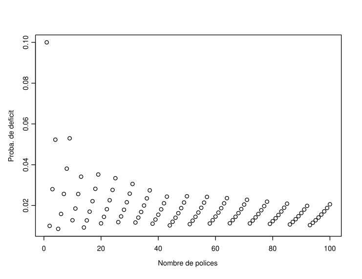
Figure 5.1: Evolution of the probability of ruin as a function of the portfolio size (\(n\)) when \(q=0.1\) and \(q=0.01\)

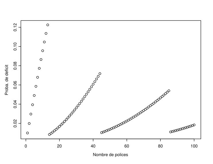
Figure 5.2: Evolution of the probability of ruin as a function of the portfolio size (\(n\)) when \(q=0.1\) and \(q=0.01\)

Now let’s consider larger values of \(n\). Figure ?? describes the evolution of the probability of ruin as a function of the portfolio size \(n\) when \(n\) varies from 1 to 100,000. Again, the same type of phenomenon can be observed, namely that the insurer needs to underwrite batches of new policies to decrease its annual deficit probability, which increases between two batches. It is also clear that the asymptotic value of 1% is consistently exceeded, especially when \(n\) is small.

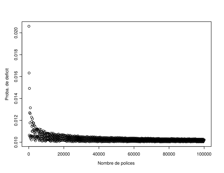
Figure 5.3: Evolution of the probability of ruin as a function of the portfolio size (\(n\)) when \(q=0.1\) and \(q=0.01\)

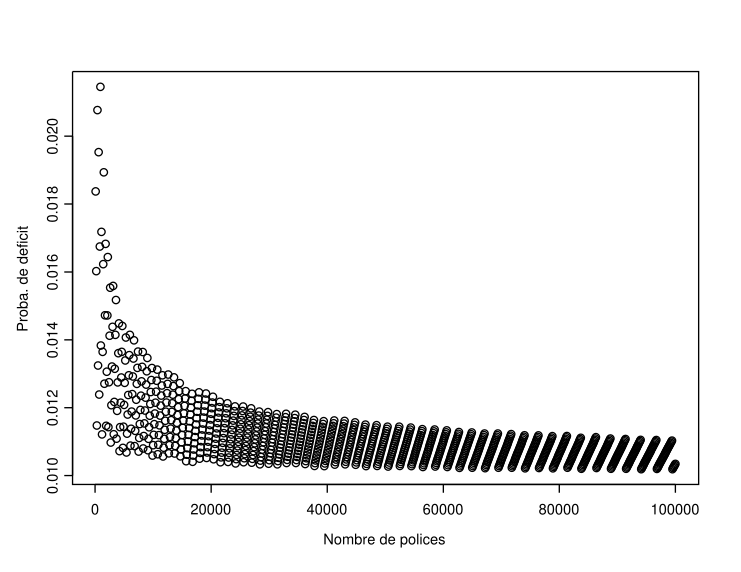
Figure 5.4: Evolution of the probability of ruin as a function of the portfolio size (\(n\)) when \(q=0.1\) and \(q=0.01\)

5.3.4 The case of indemnity-based claims

Let’s now consider the case where the annual claim amounts themselves are random; this is the case of indemnity-based claims. Consider claim amounts \(S_i\) of the form (??). In this case, \[ \sum_{i=1}^nS_i=_{\text{law}}\sum_{k=1}^NZ_k\text{ where }N\sim\mathcal{B}in(n,q). \] It’s important to emphasize that the index \(i\) on the left-hand side refers to the \(i\)-th policy in the portfolio, and the index \(k\) on the right-hand side refers to the \(k\)-th claim that affects the portfolio (without reference to the policy that generated it). Similarly, \(n\) on the left-hand side represents the number of policies in the portfolio, while \(N\) on the right-hand side represents the (random) number of claims affecting the portfolio. This prefigures the individual and collective modeling of insurance portfolios, which we will discuss in detail in Chapter 6.

If the company charges policyholders an amount equal to the pure premium and wants to limit its deficit risk to a level \(\epsilon\), it must have a capital based on the approximation of the central limit theorem \[\begin{eqnarray} \kappa_\epsilon&\approx&\sqrt{\mathbb{V}[S_1]}\sqrt{n}\Phi^{-1}(1-\epsilon)\nonumber\\ &=&\sqrt{q\mathbb{V}[Z_1]+q(1-q)\big\{\mathbb{E}[Z_1]\big\}^2}\sqrt{n}\Phi^{-1}(1-\epsilon).\tag{5.5} \end{eqnarray}\]

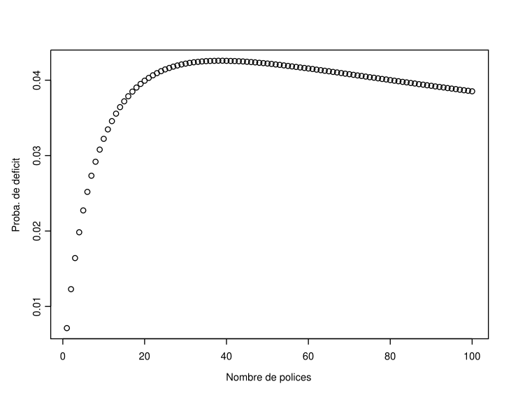
Figure 5.5: Evolution of the probability of ruin as a function of the portfolio size (\(n\)) when \(a=\tau=1\), \(q=0.01\) and \(\epsilon=1\%\)

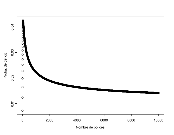
Figure 5.6: Evolution of the probability of ruin as a function of the portfolio size (\(n\)) when \(a=\tau=1\), \(q=0.01\) and \(\epsilon=1\%\)

In Figure ??, you can see the evolution of the probability of ruin as a function of the number of policies in the portfolio when \(Z_1\sim\mathcal{G}am(1,1)\) (thus \(\mathbb{E}[Z_1]=\mathbb{V}[Z_1]=1\)), \(\epsilon=1\%\), \(q=0.01\), and the capital was calculated based on the normal approximation (5.5). It’s interesting to note the growth of this probability for small values of \(n\), followed by a steady decrease. Thus, there is a minimum portfolio size beyond which the probability of ruin decreases with the number \(n\) of policies. This threshold must be reached for the insurer to reduce its risk of ruin by underwriting new policies.

5.4 Security Loading

5.4.1 Concept

In practice, insurers do not settle for the pure premium; they add a security loading to it, which is assumed to correct the discrepancies between the observed reality and the approximation induced by the law of large numbers. The term “net premium” refers to the pure premium to which the security loading has been added. The size of the security loading depends on the premium calculation principle adopted by the company.

Traditionally, this security loading is expressed as a percentage of the pure premium, so that \[ p_{\text{net}}=(1+\rho)p_{\text{pure}}, \] where \(\rho\) is referred to as the security loading rate. Note that this practice is essentially justified for its convenience and is not without question (especially due to the distortions it introduces in a segmented universe).

5.4.2 Determining the security loading Based on the Central Limit Theorem

The height of the security loading is often chosen by limiting the probability of ruin to an acceptable threshold \(\epsilon\) for the insurer, i.e., such that the inequality \[ \Pr\left[\sum_{i=1}^nS_i>(1+\rho)n\mu+\kappa\right]\leq\epsilon \] is satisfied. Then, according to the central limit theorem, \[ \Pr\left[\sum_{i=1}^nS_i>(1+\rho)n\mu+\kappa\right]\approx \overline{\Phi} \left(\frac{\rho n\mu+\kappa}{\sigma\sqrt{n}}\right), \] or equivalently, \[ \rho=\frac{\Phi^{-1}(1-\epsilon)\sigma\sqrt{n}-\kappa}{n\mu}. \] It’s noticeable that the security loading \(\rho\) increases as the chosen threshold \(\epsilon\) limiting the probability of deficit decreases. The security loading also increases with the variance of claim costs but decreases as the capital \(\kappa\) available to the company increases.

Finally, the security loading rate \(\rho\) decreases with the size \(n\) of the portfolio. As the number of policies grows, the insurer must allocate more resources to reduce the probability of deficit to \(\epsilon\), but the relative contribution of each policyholder to the formation of these resources decreases.

5.4.3 The Absolute Necessity of Security Load

An insurer subscribing to new business sees the variance of its result increase, since \[\begin{eqnarray*} \mathbb{V}\left[np+\kappa-\sum_{i=1}^nS_i\right]&=&n\sigma^2\\ &\leq &(n+1)\sigma^2\\ &=&\mathbb{V}\left[(n+1)p+\kappa-\sum_{i=1}^{n+1}S_i\right], \end{eqnarray*}\] when risks are independent. If variance is used as a decision criterion, the insurer has no incentive to underwrite new business. Even though the average cost per policy becomes less variable as the portfolio size increases (cf. \(\mathbb{V}[\overline{S}^{(n)}]=\frac{\sigma^2}{n}\) under the conditions of the law of large numbers), the overall result of the company becomes more and more variable.

Suppose \(S_i=\mu+Z_i\), where the \(Z_i\) are independent and identically distributed random variables with a normal distribution \(\mathcal{N}or(0,\sigma^2)\). If \(p=\mu\), then the probability of ruin \[ \Pr\left[\sum_{i=1}^nS_i>n\mu+\kappa\right]=\overline{\Phi}\left(\frac{\kappa}{\sigma\sqrt{n}}\right) \] increases with \(n\) and tends toward 0.5. This simple example illustrates that the annual deficit probability does not always decrease with the portfolio size \(n\). It only decreases as \(n\) increases in the above example if the insurer has added a security loading (i.e., if \(p>\mu\)). Indeed, the deficit probability then becomes \[ \Pr\left[\sum_{i=1}^nS_i>np+\kappa\right]=\overline{\Phi}\left(\frac{n(p-\mu)+\kappa}{\sigma\sqrt{n}}\right), \] which tends to 0 as \(n\to +\infty\) if \(p>\mu\). Therefore, what allows the insurer to operate is the accumulation of security loads, which absorb the variability of claims.

5.4.4 Premium Calculation Principle

5.4.4.1 Definition

A premium calculation principle is a functional \(\mathbb{H}\) that associates a net premium with (the cumulative distribution function of) a risk \(S\). It is a rule adopted by the insurance company to determine the security loading (given by \(\mathbb{H}[S]-\mathbb{E}[S]\)) and, consequently, set the price of the risk.

Remark. Premium calculation principles are closely linked to risk measures, which will be studied in the following chapter.

5.4.4.2 Desirable Properties of Premium Calculation Principles

Generally, a series of important properties are established that premium calculation principles should satisfy. Let’s detail some of these for reference:

• (P1) For any risks \(S\) and \(T\), the inequality \[ \mathbb{H}[S+T]\leq \mathbb{H}[S]+\mathbb{H}[T] \] must be satisfied. This requirement ensures that the policyholder has no incentive to split the risk. On the contrary, their premium will be reduced if they place the entire risk with the same company.
• (P2) For any risks \(S\) and \(T\), the inequality \[ \mathbb{H}[S]\leq \mathbb{H}[S+T] \] must be satisfied. This guarantees that a policy offering more protection than another must be accompanied by a higher premium.
• (P3) For any risk \(S\) for which there exists a constant \(M\) such that \(\Pr[S\leq M]=1\), the inequality \[ \mathbb{H}[S]\leq M \] must be satisfied. This condition is very natural: no rational policyholder would be willing to pay a premium greater than the maximum loss they could incur.

5.4.4.3 Examples of Premium Calculation Principles

Below, we detail some classical premium calculation principles.

::: {definition name=“Expectation Premium Principle”} According to this principle, \[ \mathbb{H}[S]=(1+\rho)\mathbb{E}[S],\hspace{2mm}\rho>0. \] :::

The expectation premium principle is the simplest one: the net premium depends only on a numerical characteristic associated with the risk, its mean, while the security loading is proportional to the mean. However, two risks \(S\) and \(T\) with the same mean can still represent very different dangers for the insurance company.

Properties P1 and P2 are trivially satisfied. However, P3 is not necessarily satisfied, as the following example shows. Consider a constant risk \(S=M\); then \[ \mathbb{H}[S]=(1+\rho)M>M. \]

::: {definition name=“Standard Deviation Premium Principle”} According to this principle, \[ \mathbb{H}[S]=\mathbb{E}[S]+\theta\sqrt{\mathbb{V}[S]},\hspace{2mm}\theta>0. \] :::

In this case, the security loading is proportional to the standard deviation of the risk, thus taking into account its variability. This principle satisfies P1 since the inequality \[\begin{equation} \sqrt{\mathbb{V}[S+T]}\leq\sqrt{\mathbb{V}[S]}+ \sqrt{\mathbb{V}[T]} \tag{5.6} \end{equation}\] is always fulfilled. Using (5.6), it follows that \[\begin{eqnarray*} \mathbb{H}[S+T] & = & \mathbb{E}[S+T]+\theta\sqrt{\mathbb{V}[S+T]}\\ & =& \mathbb{E}[S]+\mathbb{E}[T]+\theta\sqrt{\mathbb{V}[S+T]}\\ & \leq & \mathbb{E}[S]+\mathbb{E}[T]+\theta\Big\{\sqrt{\mathbb{V}[S]}+ \sqrt{\mathbb{V}[T]}\Big\}\\ & = & \mathbb{H}[S]+\mathbb{H}[T]. \end{eqnarray*}\]

P2 is not satisfied. To convince ourselves of this, let’s consider a risk \(S_p\) such that \[\begin{equation} S_p=\begin{cases} 0, & \text{with probability } 1-p,\\ M, & \text{with probability } p. \end{cases} \tag{5.7} \end{equation}\] In this case, the first two moments of \(S_p\) are given by \[ \mathbb{E}[S_p] = Mp \quad \text{and} \quad \text{Var}[S_p] = M^2p(1-p). \] Consequently, the premium demanded for coverage of \(S_p\) is \[ \mathbb{H}[S_p] = Mh(p) \quad \text{where} \quad h(p) = p+\theta\sqrt{p(1-p)}. \] Let’s take a closer look at the function \(h(\cdot)\). Through differentiation, we have \[ \frac{d}{dp}h(p) = 1+\frac{\theta(1-2p)}{2 \sqrt{p(1-p)}}, \] and it can be easily observed that \[ \lim_{p\to 1}\frac{d}{dp}h(p)=-\infty. \] As \(h\) is continuous from the left at 1 and since \(S_1=M\), there must exist a value \(p_0<1\) for which \(\mathbb{H}[S_{p_0}]>\mathbb{H}[S_1]=M\). Since \(M-S_{p_0}\geq 0\), \[ \mathbb{H}[S_{p_0}]>\mathbb{H}[S_1]=\mathbb{H}[S_{p_0}+(M-S_{p_0})], \] and P2 cannot be satisfied. Similarly, P3 is also not satisfied since \(\mathbb{H}[S_{p_0}]>M\).

Remark (Choice of $\theta$ for the standard deviation principle). Consider a portfolio of \(n\) policies, with claim amounts \(S_1,S_2,\ldots,S_n\), assumed to be independent and identically distributed. To determine the level of safety loading \(\theta\), we can require that the inequality \[ \Pr\left[\sum_{i=1}^nS_i>\sum_{i=1}^n\mathbb{H}[S_i]+\kappa\right]\leq\epsilon \] holds, ensuring that the company will only be in deficit with a very low probability \(\epsilon\). Consequently, by the central limit theorem, we have approximately \[\begin{align*} &\Pr\left[\sum_{i=1}^nS_i>\sum_{i=1}^n\mathbb{H}[S_i]+\kappa\right] \\ &\quad \approx 1-\Phi\left(\rho\frac{\sum_{i=1}^n\sqrt{\text{Var}[S_i]}}{\sqrt{\sum_{i=1}^n\text{Var}[S_i]}} +\frac{\kappa}{\sqrt{\sum_{i=1}^n\text{Var}[S_i]}}\right), \end{align*}\] leading to \[ \theta=\frac{z_\epsilon\sqrt{\text{Var}\left[\sum_{i=1}^nS_i\right]}-\kappa}{\sum_{i=1}^n\sqrt{\text{Var}[S_i]}} =\frac{z_\epsilon\sigma\sqrt{n}-\kappa}{n\sigma}. \]

5.4.5 Comments

As we can see, the current premium calculation principles have theoretical drawbacks. Nevertheless, this does not question their practical relevance, and this for two reasons: firstly, the counterexamples constructed above are relatively artificial, and secondly, companies are never obliged to cover the risks available to them. This can be important for P1, for instance. Thus, it could be imagined that a company using a principle \(\mathbb{H}\) that does not satisfy P1 refuses to separately cover the risks \(S\) and \(T\) for which \(\mathbb{H}[S+T]>\mathbb{H}[S]+\mathbb{H}[T]\). If the company adopts such a strategy, there is no longer a need to limit oneself to principles satisfying P1.

5.5 Security Coefficient

5.5.1 Company’s Technical Result

5.5.1.1 Consequences of the Bienaymé-Chebyshev Inequality

The mean of \(R\) is \[ \mathbb{E}[R] = (1+\rho)n\mu - n\mu = \rho n\mu, \] which is the sum of the safety loadings. Denoting \(\sigma^2\) as the common variance of \(S_i\), the variance of \(R\) is \[ \mathbb{V}[R] = n\sigma^2, \] due to the independence of \(S_i\).

Now, let’s define the security coefficient.

The security coefficient, denoted as \(\beta\), is defined as \[ \beta = \frac{\kappa + \rho n \mu}{\sigma\sqrt{n}}. \]

Defined this way, the security coefficient appears as the ratio between, on one hand, the average technical result of the insurer \(\mathbb{E}[R] = \rho n\mu\) increased by the capital \(\kappa\) allocated to the insurance branch, and on the other hand, the standard deviation of the insurer’s result \(R\). Thus, it is the ratio between the insurer’s safety (numerator) and the risk (denominator).

Then we have \[\begin{align*} &\Pr\Big[|R-\rho n\mu|\leq t\sigma\sqrt{n}\Big]\\ &= \Pr\Big[\rho n \mu-t\sigma\sqrt{n}\leq R\leq \rho n \mu+t\sigma\sqrt{n}\Big]\\ &> 1-\frac{1}{t^2}. \end{align*}\] Choosing \(t\) such that \[ \kappa = t\sigma\sqrt{n} - \rho n\mu \Leftrightarrow t = \beta, \] we then have \[ \Pr\Big[R<-\kappa\text{ or }R>\kappa+2\rho n\mu\Big] \leq \frac{1}{\beta^2}. \] We can see that \[ \max\Big\{\Pr[R<-\kappa], \Pr[R>\kappa+2\rho n\mu]\Big\} \leq \frac{1}{\beta^2}, \] so \(1/\beta^2\) does indeed provide an upper bound on the probability of the unfavorable event \(\{R<-\kappa\}\) and the overly favorable event \(\{R>\kappa+2\rho n\mu\}\): this illustrates the necessary stability of the insurer’s results, which cannot fall below a threshold of \(-\kappa\) without facing bankruptcy, but also cannot be too high, as the pure premium must enable the insurer to compensate for claims without excess or deficit.

5.5.2 Determining the Security Coefficient

To ensure the ability to meet its commitments, the insurer adds a safety loading to the pure premium and plans for sufficient solvency margin to deal with certain deficit periods. Note that the probability of ruin can be rewritten as \[ \Pr\left[\sum_{i=1}^nS_i-(1+\rho)n\mu > \kappa\right] = \Pr\left[\frac{\sum_{i=1}^nS_i-n\mu}{\sigma\sqrt{n}} > \underbrace{\frac{\kappa+\rho n\mu}{\sigma\sqrt{n}}}_{=\beta}\right], \] so according to the central limit theorem, the probability of ruin is approximately \[ \Pr\left[\sum_{i=1}^nS_i-(1+\rho)n\mu > \kappa\right] \approx \overline{\Phi}(\beta). \] In practice, it is often considered that \(\beta = 4\) is sufficient since \(\Phi(4) = 0.999968\), which corresponds to a deficit probability on the order of \(\overline{\Phi}(4) = 3.2 \times 10^{-5}\). This gives us \[ \rho = \frac{4\sigma\sqrt{n} - \kappa}{n\mu}. \]

5.5.3 Determining the Safety Loading Based on the Bienaymé-Chebyshev Inequality

The Bienaymé-Chebyshev inequality gives \[\begin{eqnarray*} \Pr\Big[\rho n \mu-t\sigma\sqrt{n}\leq R\leq \rho n \mu+t\sigma\sqrt{n}\Big] &>& 1-\frac{1}{t^2}. \end{eqnarray*}\] Let’s once again choose \(t=\beta\), which yields \[ \Pr\Big[R<-\kappa\text{ or }R>\kappa+2\rho n\mu\Big] \leq \frac{1}{\beta^2}. \]

If \[ 1/\beta^2 \leq \epsilon \Leftrightarrow \beta \geq 1/\sqrt{\epsilon}, \] then we will indeed have \(\Pr[R<-\kappa] \leq \epsilon\). The condition \(\beta \geq 1/\sqrt{\epsilon}\) allows us to determine \(\rho\).

5.6 The Normal-Power (NP) Approximation

In this section, we will discuss certain approximations used in reinsurance, particularly the NP (Normal Power) approximation, which improves upon the Gaussian approximation by taking into account skewness (third-order moment). The Edgeworth approximation allows for consideration of higher-order moments in a similar manner (especially kurtosis, the tail flattening coefficient). These approximations were studied in the 1930s, driven by the work of Haldane, Wilson, or Hilferty (following Edgeworth’s work at the beginning of the century), and used in insurance by Seal and Pentikäinen as early as 1977. Other numerical approximation methods (simulation methods or fast Fourier transform-based methods, in particular) will be discussed later.

5.6.1 Skewness Coefficient

5.6.1.1 Definition

The skewness coefficient is obtained by comparing the third centered moment to the cube of the standard deviation (to make it dimensionless).

Given a random variable \(X\) with mean \(\mu\) and variance \(\sigma^2\), the skewness coefficient, denoted as \(\gamma[X]\), is defined as \[ \gamma[X] = \frac{\mathbb{E}[(X-\mu)^3]}{\sigma^3} = \frac{\mathbb{E}[X^3] - 3\mathbb{E}[X]\mathbb{E}[X^2] + 2\{\mathbb{E}[X]\}^3}{\sigma^3}. \]

If the probability density of \(X\) is symmetric around the mean, then \(\gamma[X] = 0\). A positive value of \(\gamma[X]\) indicates a distribution that assigns a greater probability mass to “small” values. Conversely, a negative value of \(\gamma[X]\) indicates a distribution where a significant probability mass is concentrated on “large” values.

Skewness coefficients associated with continuous distributions are listed in Table ??.

5.6.2 Edgeworth Expansion

Let \(S\) represent the amount of claims related to an insurance policy in the portfolio, with a cumulative distribution function \(F_S\). Let’s define \[ Z=\frac{S-\mathbb{E}[S]}{\sqrt{\mathbb{V}[S]}}, \] the centered-reduced claim amount. Clearly, the cumulative distribution function \(F_Z\) of \(Z\) and the cumulative distribution function \(F_S\) of \(S\) are related by the relation \[ F_Z(x) = F_S\left(\mathbb{E}[S]+x\sqrt{\mathbb{V}[S]}\right),\hspace{2mm} x\in \mathbb{R}. \] Note that \(\mathbb{E}[Z]=0\), \(\mathbb{E}[Z^2]=1\), and \(\mathbb{E}[Z^3]=\gamma[S]\). Let \(M_Z(t)=\mathbb{E}[\exp(tZ)]\) be the moment generating function of \(Z\), and define \[ \widetilde{M}(t)=\exp(-t^2/2)M_Z(t). \] By Taylor expanding \(\widetilde{M}\) as \(\sum_{k=0}^{+\infty}a_kt^k\), we get \[\begin{equation} M_Z(t)=\sum_{k=0}^{+\infty}a_kt^k\exp(t^2/2). \tag{5.8} \end{equation}\]

Now, let’s prove the following result.

Lemma 5.1 The identity \[ t^k\exp(t^2/2)=(-1)^k\int_{z=-\infty}^{+\infty}\exp(tz) \phi^{(k)}(z)dz, \] holds for any \(t\in \mathbb{R}\) and \(k\in \mathbb{N}\), where \(\phi^{(k)}\) denotes the \(k\)th derivative of the probability density \(\phi\) associated with the \(\mathcal{N}or(0,1)\) distribution.

Proof. Let’s prove the result for \(k=0\): \[\begin{eqnarray*} &&\int_{z=-\infty}^{+\infty}\exp(tz) \phi(z)dz\\ &=&\frac{1}{\sqrt{2\pi}}\exp(t^2/2) \int_{z=-\infty}^{+\infty}\exp(-(z-t)^2/2)dz \\ &=&\exp(t^2/2). \end{eqnarray*}\] Now, let’s proceed by induction. Assume the result holds for \(k=n\). Then we have \[\begin{eqnarray*} &&\int_{z=-\infty}^{+\infty}\exp(tz) (-1)^{n+1}\phi^{(n+1)}(z)dz \\ & = & (-1)^{n+1}\left\{\left[\exp(tz)\phi^{(n)} (z)\right]_{z=-\infty}^{+\infty}\right. \\ & & \hspace{10mm}\left. -\int_{z=-\infty}^{+\infty}t\exp(tz)\phi^{(n)}(z)dz\right\} \\ & = & (-1)^nt\int_{z=-\infty}^{+\infty}\exp(tz) \phi^{(n)}(z)dz \\ & = & t^{k+1}\exp(t^2/2), \end{eqnarray*}\] which completes the proof.

Thanks to Lemma 5.1, (5.8) becomes \[\begin{eqnarray*} M_Z(t) & = & \sum_{k=0}^{+\infty}a_k \int_{z=-\infty}^{+\infty}\exp(tz) (-1)^k\phi^{(k)}(z)dz \\ & = & \int_{z=-\infty}^{+\infty}\exp(tz) \left\{\sum_{k=0}^{+\infty}a_k(-1)^k\phi^{(k)}(z)\right\}dz. \end{eqnarray*}\] Therefore, \(M_Z\) is the moment generating function of a probability distribution with density \(\sum_{k=0}^{+\infty}a_k(-1)^k\phi^{(k)}(x)\). As the moment generating function is unique, it follows that \[\begin{equation} F_Z(z)=\sum_{k=0}^{+\infty}(-1)^ka_k\Phi^{(k)}(z). \tag{5.9} \end{equation}\] Formula (\(\ref{eq:eqA2}\)) is known as the Edgeworth expansion of \(F_Z\). Emphasize the fact that (\(\ref{eq:eqA2}\)) was obtained in a very informal manner. In fact, we haven’t paid much attention to convergence issues (in fact, the series (\(\ref{eq:eqA2}\)) diverges in many cases). The Edgeworth approximation consists of truncating the series (\(\ref{eq:eqA2}\)) to a finite number of terms, say \(\nu\), i.e. using the approximation \[ F_Z(z)\approx \sum_{k=0}^\nu(-1)^ka_k\Phi^{(k)}(z). \] By definition, \[ a_k=\frac{1}{k!}\widetilde{M}^{(k)}(0),\hspace{2mm}k=0,1,2,\ldots, \] so that \[\begin{eqnarray*} a_0 & = & 1,\\ a_1 & = & 0,\\ a_2 & = & 0,\\ a_3 & = & \frac{\mathbb{E}[Z^3]}{6}, \\ a_4 & = & \frac{\mathbb{E}[Z^4]-3}{24},\\ a_5 & = & 0, \\ a_6 & = & \frac{(\mathbb{E}[Z^3])^2}{72}. \end{eqnarray*}\] Thus, for \(\nu=6\), the Edgeworth approximation reduces to \[\begin{eqnarray} F_Z(z)&\approx&\Phi(z)-\frac{\mathbb{E}[Z^3]}{6}\Phi^{(3)}(z)+ \frac{\mathbb{E}[Z^4]-3}{24}\Phi^{(4)}(z)\nonumber\\ &&+\frac{(\mathbb{E}[Z^3])^2}{72} \Phi^{(6)}(z). \tag{5.10} \end{eqnarray}\] Often, only the first two terms of (5.10) are used, yielding \[\begin{equation} F_S(x)\approx\Phi\left(\frac{x-\mathbb{E}[S]}{\sqrt{\mathbb{V}[S]}}\right) -\frac{\gamma[S]}{6}\Phi^{(3)}\left(\frac{x-\mathbb{E}[S]}{\sqrt{\mathbb{V}[S]}}\right). \tag{5.11} \end{equation}\] As \[\begin{eqnarray*} \Phi^{(1)} (z) &=& \frac{1}{\sqrt{2 \pi}} \exp (-z^2/2),\\ \Phi^{(2)} (z) &=& \frac{-1}{\sqrt{2 \pi}} z \exp (-z^2/2),\\ \Phi^{(3)} (z) &=& \frac{1}{\sqrt{2 \pi}} \Big(- \exp (- z^2/2) + z^2 \exp (- z^2/2)\Big)\\ &=&(z^2-1)\Phi^{(1)}(z), \end{eqnarray*}\] the approximation (5.11) can be rewritten as \[\begin{equation} F_S(x)\approx\Phi\left(\frac{x-\mathbb{E}[S]}{\sqrt{\mathbb{V}[S]}}\right) -\frac{\gamma[S]}{6}\left(\left(\frac{x-\mathbb{E}[S]}{\sqrt{\mathbb{V}[S]}}\right)^2-1\right) \phi\left(\frac{x-\mathbb{E}[S]}{\sqrt{\mathbb{V}[S]}}\right). \tag{5.12} \end{equation}\]

Remark. It is interesting to make the following comments:

1. As soon as more than one term is used in the Edgeworth approximation, negative values can be obtained for certain values of \(z\). Thus, the approximation provided in (5.10) or (5.11) is not a cumulative distribution function.
2. The approximation provided by (5.10) is generally good when \(z\) is close to 0. However, the error grows rapidly as \(|z|\) increases. In other words, the Edgeworth approximation (5.12) is considered good around the mean, but deteriorates significantly in the tails of the distribution. A clever way to avoid this drawback is to use the Esscher transform, presented later.
3. As the Edgeworth series often diverges, adding an extra term doesn’t necessarily improve the quality of the approximation.

5.6.3 Esscher Approximation

5.6.3.1 Esscher Transformation

The Esscher transformation is defined for distributions possessing a moment-generating function (also known as Cramér distributions in risk theory). It involves replacing the original distribution with another distribution that is more severe for the insurer. When used in conjunction with the Edgeworth approximation, the Esscher technique often yields accurate approximations.

Let \(S\) be a real random variable with distribution function \(F_S\) and moment-generating function \(M_S\). For each \(h\in{\mathbb{R}}\), associate a random variable \(S_h\) with distribution function \(F_h\) defined by \[\begin{equation} F_h(t)=\frac{1}{M_S(h)}\int_{\xi=-\infty}^t\exp(h\xi)dF_S(\xi). \tag{5.13} \end{equation}\] The distribution function \(F_h\) is called the Esscher transform of \(F_S\) with parameter \(h\).

::: {proposition #FGMEsscher} It is easy to see that the moment-generating function \(M_h\) associated with the distribution function \(F_h\) is given by \[\begin{eqnarray*} M_h(t)&=&\mathbb{E}[\exp(tS_h)]\\ &=&\frac{1}{M_S(h)}\int_{s\in{\mathbb{R}}}\exp\big((h+t)s\big)dF_S(s)\\ &=&\frac{M_S(t+h)}{M_S(h)}. \end{eqnarray*}\] :::

Example 5.3 Consider \(N\sim\mathcal{P}oi(\lambda)\) and let’s focus on the distribution of \(N_h\). To do this, let’s calculate its moment-generating function, given according to Property \(\ref{FGMEsscher}\) by \[\begin{eqnarray*} M_h(t)&=&\frac{\mathbb{E}[\exp((t+h)N)]}{\mathbb{E}[\exp(hN)]}\\ &=&\frac{\varphi_N(\exp(t+h))}{\varphi_N(\exp(h))}\\ &=&\frac{\exp\Big(\lambda(\exp(t+h)-1)\Big)}{\exp\Big(\lambda(\exp(h)-1)\Big)}\\ &=&\exp\Big(\lambda \exp(h)(\exp(t)-1)\Big) \end{eqnarray*}\] where we recognize the moment-generating function associated with the Poisson distribution with mean \(\lambda\exp(h)\). Thus, \(N_h\sim\mathcal{P}oi(\lambda\exp(h))\).

5.6.3.2 Esscher Transformation and Pure Premium

The Esscher transformation does not affect the support of \(S\): thus, \(S\) and \(S_h\) take values in the same set. However, the values of \(S_h\) are more towards the right as \(h\) increases, as shown by the following result (we will revisit this aspect in Chapter \(\ref{ChapMicroEcon}\)).

Proposition 5.1 \(\mathbb{E}[S_h]\) is an increasing function of \(h\).

Proof. Indeed, \[ \mathbb{E}[S_h]=M_h'(0)=\frac{M_S'(h)}{M_S(h)} \] from which we derive \[\begin{eqnarray*} \frac{d}{dh}\mathbb{E}[S_h]&=&\frac{M_S''(h)M_S(h)-\{M_S'(h)\}^2}{\{M_S(h)\}^2}\\ &=&M_h''(0)-\{M_h'(0)\}^2=\mathbb{V}[S_h]>0. \end{eqnarray*}\]

5.6.3.3 Esscher Approximation

Now let’s demonstrate the utility of the Esscher transformation for actuaries. Suppose we are interested in \(F_S(x)=\Pr[S\leq x]\) for a certain value of \(x\). The main idea of the Esscher method is to choose \(h\) such that \[ \mathbb{E}[S_h]=\frac{M_S'(h)}{M_S(h)}=x \] and then apply the Edgeworth approximation (5.11) to \(S_h\) rather than \(S\). This leads to \[\begin{equation} f_h(y)dy\approx\phi(z)dz-\frac{\mathbb{E}[(S_h-x)^3]}{6\{\mathbb{V}[S_h]\}^{3/2}}\phi^{(3)}(z)dz, \tag{5.14} \end{equation}\] where \[ z=\frac{y-x}{\sqrt{\mathbb{V}[S_h]}}. \] Returning to (5.13), we see that \[ f_S(y)=M_S(h)f_h(y)\exp(-hy), \] which upon integration yields \[\begin{equation} \overline{F}_S(x)=M_S(h)\int_{y=x}^{+\infty}\exp(-hy)f_h(y)dy, \tag{5.15} \end{equation}\] and \[\begin{equation} F_S(x)=M_S(h)\int_{y=-\infty}^x\exp(-hy)f_h(y)dy. \tag{5.16} \end{equation}\] The question now is whether it is better to insert the approximation (5.14) into (5.15) or into (5.16) to obtain the desired approximation for \(F_S(x)\). The answer to this question depends on the sign of \(h\):

1.If \(h>0\) (i.e. \(x>\mathbb{E}[S]\)), using (5.15) is preferable; 2. If \(h<0\) (i.e. \(x<\mathbb{E}[S]\)), (5.16) should yield better results.

5.6.3.4 NP Approximation

Due to the limited applicability of the Edgeworth expansion (which provides a reasonable approximation only around the mean), actuaries have proposed the NP method. This method serves as an alternative to using both the Edgeworth and Esscher approximations described above together.

Starting with the approximation (5.10) limited to the first two terms: \[ F_Z(z)\approx\Phi(z)-\frac{\mathbb{E}[Z^3]}{6}\Phi^{(3)}(z). \] The above approximation can actually be expressed as: \[ F_Z(z)\approx\Phi(z)-\frac{\mathbb{E}[Z^3]}{6}(z^2-1)\Phi^{(1)}(z). \] Now, using a Taylor expansion, we have \[\begin{eqnarray*} F_Z(z+\Delta z) & \approx & F_Z(z)+f_Z(z)\Delta z \\ & \approx & \Phi(z)-\frac{\mathbb{E}[Z^3]}{6}(z^2-1)\Phi^{(1)}(z) +\Phi^{(1)}(z)\Delta z, \end{eqnarray*}\] which ultimately gives the formula \[ F_Z(z+\Delta z)\approx\Phi(z)-\left(\frac{\mathbb{E}[Z^3]}{6}(z^2-1)-\Delta z \right)\Phi^{(1)}(z). \] By setting \(\Delta z=\mathbb{E}[Z^3](z^2-1)/6\), the coefficient of \(\Phi^{(1)}(z)\) cancels out, leaving only \[ F_Z\left(z+\frac{\mathbb{E}[Z^3]}{6}(z^2-1)\right)\approx\Phi(z); \] this latter relation is known as the NP (“Normal Power”) approximation.

Remark. Note that when \(\mathbb{E}[Z^3]=0\), the NP approximation reduces to assuming that \(S\) follows a normal distribution.

Assuming \(\mathbb{E}[Z^3]\neq 0\), let’s seek an approximation for \(F_Z(y)\). We have \[ F_Z(y)\approx\Phi(z) \] where \(z\) satisfies \[ z+\frac{\mathbb{E}[Z^3]}{6}(z^2-1)=y \] and hence \[ z=\sqrt{\frac{9}{(\mathbb{E}[Z^3])^2}+1+\frac{6}{\mathbb{E}[Z^3]}y}-\frac{3}{\mathbb{E}[Z^3]}, \] as long as the term under the square root is non-negative. The approximation for \(F_S\) follows immediately by substituting \[ y=\frac{x-\mathbb{E}[S]}{\sqrt{\mathbb{V}[S]}}, \] yielding \[ F_S(x)\approx\Phi\left(\frac{-3}{\gamma[S]} +\sqrt{\frac{9}{(\gamma[S])^2}+1+\frac{6(x-\mathbb{E}[S])} {\gamma[S]\sqrt{\mathbb{V}[S]}}}\right), \] which is valid for \[ x>\mathbb{E}[S]+\sqrt{\mathbb{V}[S]}, \] and sufficiently accurate as long as \(0\leq \gamma[S]\leq 2\); the quality of the approximation diminishes as \(\gamma_S\) increases.

5.6.3.5 NP Approximation of Quantiles

The NP approximation also allows for the approximation of quantiles of \(S\). If \(z_\alpha\) represents the \(100(1-\alpha)\)th quantile of the standard normal distribution, we have \[\begin{eqnarray*} 1-\alpha & = & \Phi(z_\alpha) \\ & \approx & F_Z\left(z_\alpha+\frac{\mathbb{E}[Z^3]}{6}(z_\alpha^2-1)\right)\\ & = & F_S\left(\mathbb{E}[S]+\sqrt{\mathbb{V}[S]} \left(z_\alpha+\frac{\mathbb{E}[Z^3]}{6}(z_\alpha^2-1)\right) \right) \\ & = & F_S\left(\mathbb{E}[S]+\sqrt{\mathbb{V}[S]} \left(z_\alpha+\frac{\gamma[S]}{6}(z_\alpha^2-1)\right) \right), \\ \end{eqnarray*}\] providing the following approximation for the quantile \(q_{1-\alpha}\) of \(S\) \[\begin{equation} q_{1-\alpha}\approx \mathbb{E}[S]+\sqrt{\mathbb{V}[S]} \left(z_\alpha+\frac{\gamma[S]}{6}(z_\alpha^2-1)\right). \tag{5.17} \end{equation}\]

Example 5.4 (Calculation of Solvency Margin) The NP approximation can be used to estimate the minimum amount of technical provisions for non-life insurance lines. Let \(S\) be the total amount of claims related to the policies that the company has underwritten. Regulatory authorities require that the amount of technical provisions ensures the company’s solvency with a probability of \(1-\epsilon\): the amount \(\kappa_\epsilon\) of provisions must satisfy \[ \Pr[S>\kappa_\epsilon]\leq\epsilon. \] In other words, \(\kappa_\epsilon\) must be at least equal to \(\kappa_{\min}\) where \[ \Pr[S>\kappa_{\min}]=\epsilon. \] The NP approximation allows evaluating \(\kappa_{\min}\) as \[ \kappa_{\min}\approx \mathbb{E}[S]+\sqrt{\mathbb{V}[S]}\left(z_\epsilon+ \frac{\gamma[S]}{6}(z_\epsilon^2-1)\right). \]

Example 5.5 (Quantiles of Compound Poisson Distributions) The NP approximation is often used with \(S=\sum_{i=1}^NX_i\sim\mathcal{CP}oi(\lambda,F_X)\). In this case, \[ \mathbb{E}[S]=\lambda \mathbb{E}[X_1],\hspace{2mm}\mathbb{V}[S] =\lambda \mathbb{E}[X_1^2], \] and \[ \mathbb{E}\Big(S-\mathbb{E}[S]\Big)^3=\lambda \mathbb{E}[X_1^3], \] so that the quantile \(q_{1-\alpha}\) of \(S\) is approximated by \[ q_{1-\alpha}\approx\lambda \mathbb{E}[X_1]+z_\alpha\sqrt{\lambda \mathbb{E}[X_1^2]}+\frac{1}{6}(z_\alpha^2-1)\frac{\mathbb{E}[X_1^3]}{\mathbb{E}[X_1^2]}. \] This approximation is considered to be of good quality as long as \[ \gamma[S]=\frac{\mathbb{E}\Big[\Big(S-\mathbb{E}[S]\Big)^3\Big]}{(\mathbb{V}[S])^{3/2}} =\frac{\mathbb{E}[X_1^3]}{\sqrt{\lambda}(\mathbb{E}[X_1^2])^{3/2}}\leq 2. \]

5.6.3.6 NP Approximation of Stop-Loss Premiums

Let’s begin by establishing the expression of stop-loss premiums associated with the normal distribution. Consider $Yor( 0,1) $, and $X=Y+or( ,^{2}) $. Then, \[\begin{eqnarray*} \mathbb{E}\left[ \left( X-d\right)_{+}\right] &=&\mathbb{E}\left[ \left( \sigma Y+\mu -d\right)_{+}\right] \\ &=&\sigma \mathbb{E}\left[ \left( Y-\frac{d-\mu }{\sigma }\right)_{+}\right]. \end{eqnarray*}\]% We can then compute the stop-loss premium in the case of the standard normal distribution and deduce the result in the general case. The stop-loss premium associated with \(Y\) is then \[\begin{eqnarray*} \mathbb{E}\left[ \left( Y-d \right)_{+}\right] &=&\int_{y\in{\mathbb{R}}% }\left( y-d\right)_{+}\phi \left( y\right) dy \\ &=&\int_{d }^{+\infty }\left( y-d\right) \phi \left( y\right) dy\\ &=&\int_{d }^{+\infty }y\phi \left( y\right) dy-d \int_{d}^{+\infty }\phi \left( y\right) dy \\ &=&\phi \left( d \right) -d\overline{\Phi} \left( d\right), \end{eqnarray*}\]% since $’( t) =t( t) $. The stop-loss premium for \(X\) is then obtained from \[\begin{equation*} \mathbb{E}[ \left( X-d\right)_+] =\sigma \phi \left( \frac{% d-\mu }{\sigma }\right) -\left( d-\mu \right)\overline{\Phi} \left( \frac{% d-\mu }{\sigma }\right). \end{equation*}\]

Now, let’s define \[ a\left( s\right) =s+\frac{\gamma[X]}{6}\left( s^{2}-1\right), \] and \[ b\left( t\right) =-\frac{3}{\gamma[X]}+\sqrt{\frac{9}{\gamma[X]^{2}}+1+% \frac{6}{\gamma[X]}t}. \] It’s easy to notice that these functions are inverses of each other, meaning they satisfy \[ a\left( b\left( t\right) \right) =t\text{ and }b\left( a\left( u\right) \right) =u, \] and these functions are monotonic, increasing, such that \[ a\left( s\right) \geq t\Leftrightarrow b\left( t\right) \leq s. \]

Let \(Z\) be a standardized normal random variable, i.e. $ _{Z}=0 $, \(\sigma _{Z}=1\). The \(NP\) approximation applied to \(Z\) is% \[\begin{equation*} \Pr[ Z\leq a\left( z\right) ] =\Pr[b\left( Z\right) \leq z] \thickapprox \Phi \left( z\right) \text{,} \end{equation*}\]% which, in terms of tail probability, is% \[\begin{equation*} \Pr[ Z> a\left( z\right) ] =\Pr[b\left( Z\right) > z] \thickapprox \overline{\Phi} \left( z\right). \end{equation*}\]% Let \(Y\sim\mathcal{N}or(0,1)\), and define \[\begin{equation*} Y^{\ast }=a\left( \max \left\{ Y,1\right\} \right)=\left\{ \begin{array}{ll} a\left( Y\right), & \text{if }Y\geq 1, \\ 1, & \text{otherwise},% \end{array}% \right. \end{equation*}\]% then% \[\begin{equation*} \Pr[ Y^{\ast }>a\left( z\right)] =\Pr[Y>z] \thickapprox 1-\Phi \left( z\right), \text{ if }z\geq 1, \end{equation*}\]% and thus, finally, considering the fact that the \(NP\) approximation assumes that \(Z\) can be approximated by $a( Y) $ where \(Y\) is a Gaussian variable (as long as \(Y\geq 1\))\(,\) i.e.  \[ \Pr[ Z\leq s] \thickapprox \Pr[ Y^{\ast }\leq s]. \] We then obtain% \[\begin{equation*} \Pr[Z>s] \thickapprox \Pr[Y^{\ast }>s] \thickapprox 1-\Phi \left( b\left( s\right) \right), \text{ for all }s\geq 1. \end{equation*}\]

The stop-loss premium associated with \(Z\) can be written as \[\begin{eqnarray*} \mathbb{E}[ \left( Z-d\right)_{+}] &=&\int_{d}^{\infty }\Pr[ Z>s] ds\\ &\thickapprox &\int_{d}^{\infty }\Pr[Y^{\ast}>s] ds\\ &=&\mathbb{E}[ \left( Y^{\ast }-d\right)_{+}] \\ &=&\int_{{\mathbb{R}}}\left( a\left( \max \left\{ y,1\right\} \right) -1\right) _{+}\phi \left( y\right) dy \\ &=&\int_{b\left( d\right) }^{+\infty }\left( a\left( y\right) -d\right) \phi \left( y\right) dy\\ &=&\int_{b\left( d\right) }^{+\infty }\left( y+\frac{\gamma[Z]}{6}\left( y^{2}-1\right) -d\right) \phi \left( y\right) dy \\ &=&\int_{b\left( d\right) }^{+\infty }\frac{\gamma[Z]}{6}\left( y^{2}-1\right) \phi \left( y\right) dy+\int_{b\left( d\right) }^{+\infty }y\phi \left( y\right) dy\\ &&-d\int_{b\left( d\right) }^{+\infty }\phi \left( y\right) dy, \end{eqnarray*}\] from which finally, \[\begin{equation*} \mathbb{E}[ \left( Z-d\right)_{+}] \thickapprox \frac{\gamma[Z] }{6}b\left( d\right) \phi \left( b\left( d\right) \right) +\phi \left( b\left( d\right) \right) -d\big( 1-\Phi \left( b\left( d\right) \right)\big). \end{equation*}\]

The stop-loss premium for the variable \(X\sim\mathcal{N}or(\mu,\sigma^2)\) is then given by, \[\begin{eqnarray*} \mathbb{E}[ \left( X-d\right) _{+}] &\thickapprox & \sigma _{X}\frac{% \gamma[X]}{6}b\left( \frac{d-\mu _{X}}{\sigma _{X}}\right) \phi \left( b\left( \frac{d-\mu _{X}}{\sigma _{X}}\right) \right) \\ &&+\sigma _{X}\phi \left( b\left( \frac{d-\mu _{X}}{\sigma _{X}}\right) \right) \\ &&-\left( d-\mu _{X}\right) \left\{ 1-\Phi \left( b\left( \frac{d-\mu _{X}}{\sigma _{X}}% \right) \right) \right\}. \end{eqnarray*}\]

5.6.3.7 Determination of the Safety Loading Based on the NP Approximation

5.7 Using the NP Approximation to Determine the Safety Loading Rate \(\rho\) in the Expected Value Principle

The NP approximation can also be employed to fix the safety loading rate \(\rho\) appearing in the principle of mathematical expectation. Specifically, from the approximation (5.17), we deduce that \[\begin{align} \Pr\left[\sum_{i=1}^nS_i>(1+\rho)n\mu+\kappa\right]=\epsilon \\ \Rightarrow (1+\rho)n\mu+\kappa\approx n\mu+\sqrt{n}\sigma\left(z_\epsilon+ \frac{\gamma[S]}{6}(z_\epsilon^2-1)\right) \end{align}\] which allows us to derive an approximation for \(\rho\) as follows: \[\begin{align} \rho\approx\frac{\sqrt{n}\sigma\left(z_\epsilon+\frac{\gamma[S]}{6}(z_\epsilon^2-1)\right)-\kappa} {n\mu}. \end{align}\]

5.7.1 Concluding Remarks on Esscher and NP Approximations

Although the practical implications of the Esscher and NP formulas are likely fewer nowadays compared to the past (particularly due to the rise of numerical methods, notably simulation, which are widely used today and will be detailed in the final chapter), these approximations remain quite valuable for the following reasons:

1. These approximations are easy to compute and rapidly provide insights into the solution of the considered problem.
2. The techniques underlying the Esscher approximation often contribute to enhancing simulation methods.
3. The NP approximation can be incorporated into simulation programs for the entire company (or even the group) within the framework of Dynamic Financial Analysis (DFA) to account for claims experience.

5.8 The Premium

Unfortunately, the transfer of risk from the insured to the company cannot occur without cost. Added to the net premium are the portion of the company’s overhead costs plus the profit that the insurer intends to retain; the sum yields the commercial premium, or tariff premium, that the insured must pay to access the coverage offered by the insurer. Therefore, the commercial premium enables the insurer to fulfill its commitment to settle claims and also to cover its administrative costs and generate profits.

The company’s overhead costs encompass contract acquisition expenses (compensation for intermediaries), premium collection expenses, management costs (rent, employee compensation, expert and legal fees, etc.), and taxes.

Certain expenses are essential for the proper functioning of insurance. For instance, reducing claims assessment efforts leads to either an increase in fraud or a loss of quality in the matching of claims costs and indemnities. In both cases, policyholders suffer.

Lastly, the mechanism for determining the commercial premium also involves marketing considerations. There’s no reason to offer a product at a lower price than what the consumer is willing to pay. Conversely, the company might decide to significantly reduce its profit margins in a market niche it aims to dominate. It’s evident that we are departing from the technical realm and entering the domain of commercial endeavors, where authors are careful not to lead their dear readers.

5.9 Calculation of the Commercial Premium

Concretely, the commercial premium \(p_{\text{com}}\) is obtained using the following formula: \[\begin{eqnarray*} p_{\text{com}} &=& p_{\text{net}} + \text{overhead costs} + \text{commissions} \\ && + \text{anticipated profits} + \text{taxes}. \end{eqnarray*}\] To gain an understanding of the relative significance of the different components of the commercial premium, reference can be made to Table \(\ref{ComPrimComm}\).

Quite often in practice, all these loadings are calculated proportionally to the net premium. However, these proportional loadings are highly debatable in certain cases. It’s not clear why a broker or an agent should be better compensated if they bring in a risky case (corresponding to a high net premium), or why aggravated risks (such as young drivers) should contribute more to the profit or overhead costs than others.

5.10 Exercises

Exercise 5.1 The amount of a claim caused by a policy in the portfolio takes the form: \[ S=\left\{ \begin{array}{l} 0\text{ with probability }0.9\\ X\text{ with probability }0.1 \end{array} \right. \] where \[ \Pr[X>x]=\left(\frac{1}{x+1}\right)^{3/2},\hspace{2mm}x>0. \]

1. Calculate the pure premium for this policy.
2. Calculate the amount of the net premium in such a way that the probability that the amount of the claim \(S\) exceeds this amount is at most 1%.

Exercise 5.2 An insurer has a portfolio of \(n\) policies, where the annual costs of claims \(S_1,\ldots,S_n\) are independent and identically distributed, with a mean of 200 and a standard deviation of 2000. The insurer has a capital of \(\kappa\) and prices based on the principle of mathematical expectation, with a rate of \(\varrho\).

1. What is the safety loading factor \(\beta\) when \(\kappa=100000\), \(\varrho=5\%\), and \(n=5000\)? How do you assess the insurer’s situation?
2. We want to achieve \(\beta\geq 4\). To do this:

• What should the capital \(\kappa\) be for \(\varrho=5\%\) and \(n=5000\)?
• What should the loading rate \(\varrho\) be for \(\kappa=100000\) and \(n=5000\)?
• What is the minimum number of policies in the portfolio required for \(\kappa=100000\) and \(\varrho=5\%\)?

3. In light of the previous question, what do you advise the insurer to achieve \(\beta\geq 4\)?

Exercise 5.3 The total claim amount \(S\) for an insurance portfolio is given by \(S=\sum_{i=1}^NX_i\), where \(N\sim\mathcal{P}oi(\lambda)\) and \(X_i\) are independent and identically distributed exponential random variables with parameter \(\theta\). The \(X_i\) and \(N\) are also assumed to be independent.

1. Calculate the pure premium for the portfolio.
2. at most \(\epsilon\) if the insurer has capital \(\kappa\):

• based on the central limit theorem.
• based on the NP approximation.

Exercise 5.4 Consider a portfolio of 10,000 policies, where the annual total claim amount \(S\) has the following mean, variance, and skewness: \[ \mathbb{E}[S]=10\hspace{1mm}000,\hspace{2mm}\mathbb{V}[S]=1\hspace{1mm}000\hspace{1mm}000, \text{ and }\gamma[S]=2. \]

1. Calculate the probability that \(S\) exceeds 15,000:

• using the central limit theorem;
• using the Normal-Power approximation.

2. Comment on the two answers you obtained.
3. Calculate the threshold above which \(S\) will not exceed with a probability of 0.1% (i.e., the 0.999 quantile of \(S\)):

• using the central limit theorem;
• using the Normal-Power approximation.

4. Comment on the two answers you obtained. (Reminder: the 0.999 quantile of the standard normal distribution is 3.09)

Exercise 5.5

1. Show that for any positive random variable \(S\) with mean \(\mu\) and variance \(\sigma^2\), \[ \overline{F}_S(x)\leq\left\{ \begin{array}{l} \frac{1}{1+\left(\frac{x-\mu}{\sigma}\right)^2}\text{ if }x>\mu+\frac{\sigma^2}{\mu}\\ \frac{\mu}{x}\text{ if }\mu<x<\mu+\frac{\sigma^2}{\mu}. \end{array} \right. \]
2. By applying these inequalities to the total claim amount \(S=\sum_{i=1}^nS_i\), show that the inequality \[ \Pr\left[\sum_{i=1}^nS_i>\kappa+(1+\rho)n\mu\right]\leq\frac{1}{1+\beta^2} \] is valid provided that \[ \kappa+(1+\rho)n\mu>n\mu+\frac{\sigma^2}{\mu}\Leftrightarrow \beta>\frac{\sigma}{\sqrt{n}\mu}\Leftrightarrow \beta>CV[\overline{S}^{(n)}]. \]

5.11 Bibliographical Notes

Readers can refer to the books mentioned at the end of the previous chapter for more details, namely (Beard and Pentikäinen 1984), (Borch 1990), (Bühlmann 2007),(Daykin, Pentikainen, and Pesonen 1993), (Gerber 1979), (Pétauton 2000), (Seal 1969), (Straub and Actuaries (Zürich) 1988), (Sundt 1999), and (Tosetti et al. 2000).

The principles of premium calculation are now a separate branch of actuarial mathematics. It is not the objective of this chapter to exhaust the subject by any means. Readers can refer to (M. Goovaerts, De Vylder, and Haezendonck 1984) and (M. J. Goovaerts et al. 1990) for more detailed information. However, it is worth noting that despite all the mathematical developments (sometimes quite sophisticated), the premium calculation principles used in practice often remain limited to those succinctly presented in Section 5.4.4.

References

Beard, Robert, and M. Pentikäinen T. And Pesonen. 1984. Risk Theory: The Stochastic Basis of Insurance. Springer.

Borch, Karl. 1990. Economics of Insurance. Springer.

Bühlmann, Hans. 2007. Mathematical Methods in Risk Theory. Vol. 172. Springer.

Daykin, Chris D, Teivo Pentikainen, and Martti Pesonen. 1993. Practical Risk Theory for Actuaries. CRC Press.

Gerber, Hans. 1979. An Introduction to Mathematical Risk Theory. Huebner Foundation for Insurance Education.

Goovaerts, Marc J, Rob Kaas, AE Van Heerwaarden, Thierry Bauwelinckx, et al. 1990. Effective Actuarial Methods. Amsterdam-North-Holland.

Goovaerts, Marc, Florent Etienne De Vylder, and Jean Haezendonck. 1984. Insurance Premiums: Theory and Applications. North-Holland.

Pétauton, Pierre. 2000. Théorie de l’assurance Dommages. Dunod.

Seal, Hilary L. 1969. Stochastic Theory of a Risk Business. Wiley.

Straub, Erwin, and Swiss Association of Actuaries (Zürich). 1988. Non-Life Insurance Mathematics. Springer.

Sundt, Bjørn. 1999. An Introduction to Non-Life Insurance Mathematics. Vol. 28. VVW GmbH.

Tosetti, Alain, Thomas Béhar, Michel Fromenteau, and Stéphane Ménart. 2000. Assurance: Comptabilité réglementation Actuariat. Economica.