Chapter 6 Measurement and Comparison of Risks
6.1 Introduction
6.1.1 Measuring Risk: An Essential Task for Actuaries
Measuring risk is undoubtedly one of the most common tasks for actuaries. In fact, it is at the very essence of the profession. Among the measures of risk are, of course, premiums: the amount of the premium must always be proportionate to the risk, thus reflecting the danger associated with the risk transferred to the insurer. Other risk measures attempt to assess the level of economic capital. This is the capital that the company must have in order to be able to compensate for losses. As we saw in Chapter ??, this capital can be determined by limiting the probability of ruin of the insurer to a sufficiently low level. This is the approach based on Value-at-Risk, which we will detail later. We will see that this approach is not without criticism. Indeed, it does not take into account the magnitude of the deficit when ruin occurs. To address this issue, we will turn to tail expectation or Tail Value-at-Risk. This involves determining the capital in a way that can cover the worst scenarios on average.
6.1.2 Comparing Risks: Another Specialty of Actuaries
Throughout history, actuaries have also been concerned with comparing risks. To do this, they have often relied on scalar measures of the inherent danger of a risk \(X\), considering one risk more advantageous than another if the value taken by this measure on this risk is the lowest. Of course, summarizing the entire behavior of a risk in a single scalar measure, no matter how well chosen, often leads to very basic comparisons. This is why actuaries have felt the need to use more sophisticated methods of comparison, some inspired by the expected utility theory of economists (which we will present in a chapter dedicated to economic models of insurance) and others by the simultaneous use of several risk measures.
6.2 Risk Measures
6.2.1 Definition
Let’s start by precisely defining what is meant by a risk measure in this chapter.
Definition 6.1 A risk measure is a functional \(\varrho\) that assigns a positive number, denoted \(\varrho[X]\), possibly infinity, to a risk \(X\).
The idea is that \(\varrho\) quantifies the level of inherent danger of the risk \(X\): large values of \(\varrho[X]\) will indicate that \(X\) is “dangerous” (in a sense to be specified).
Henceforth, we consider \(\varrho[X]\) as the amount of capital that the company must have in order to face a financial loss of amount \(X\). More precisely, as long as \(\varrho\) is normalized, i.e. \[ \varrho[0]=0, \] \(\varrho[X]\) is the minimum amount that, added to the loss \(X\) at the beginning of the period, makes the coverage of \(X\) “acceptable”. The company must therefore have the amount \(\varrho[X]\), which is partly composed of the premiums paid by the insured and, for the rest, by the contribution of capital from the shareholders.
6.2.2 Coherence
It is generally accepted that a risk measure must satisfy certain conditions to be useful in applications. This leads to the notion of a coherent risk measure (artzner1999coherent?).
Definition 6.2 A risk measure is said to be coherent when it possesses the following properties:
- (Axiom 1 (translation invariance)) \(\varrho[X+c]=\varrho[X]+c\) for any risk \(X\) and any constant \(c\). Translation invariance guarantees that \[ \varrho\big[X-\varrho[X]\big]=0. \] Moreover, regardless of the constant \(c\), we should have \[ \varrho[c]=c. \]
- (Axiom 2 (sub-additivity)) \(\varrho[X+Y]\leq \varrho[X]+\varrho[Y]\) for any risks \(X\) and \(Y\). Sub-additivity reflects risk reduction through diversification. The effect of diversification is then measured by \[ \varrho[X]+\varrho[Y]-\varrho[X+Y]\geq 0, \] which represents the capital economy achieved by simultaneously covering risks \(X\) and \(Y\). Additivity is said to occur when there is equality, i.e. \(\varrho[X+Y]=\varrho[X]+\varrho[Y]\) for any risks \(X\) and \(Y\). In this case, the effect of diversification is null.
- (Axiom 3 (homogeneity):) \(\varrho[cX]=c\varrho[X]\) for any risk \(X\) and any positive constant \(c\). Homogeneity is often associated with a certain invariance with respect to monetary units (if we measure financial loss in millions of euros rather than thousands, the risk is not changed and the capital undergoes the same transformation). Homogeneity can also be seen as a limiting case of sub-additivity, when no diversification is possible. Indeed, if we assume that \(c\) is a positive integer, the homogeneity property ensures that \[\begin{eqnarray*} \varrho[cX]&=&\varrho[\underbrace{X+X+\ldots+X}_{c\text{ terms}}]\\ &=&\varrho[X]+\varrho[X]+\ldots+\varrho[X]=c\varrho[X]. \end{eqnarray*}\]
- (Axiom 4 (Monotonicity)) \(\Pr[X\leq Y]=1\Rightarrow\varrho[X]\leq\varrho[Y]\) for any risks \(X\) and \(Y\). This property expresses the fact that more capital is needed when the financial loss becomes more severe. It is therefore very natural. \end{description}
Remark. In the context of risk theory, risk measures must also include a loading for safety, meaning that they must satisfy the inequality \[ \varrho[X]\geq\mathbb{E}[X] \] for any risk \(X\). The minimum capital must exceed the expected loss, otherwise ruin becomes certain (under the conditions of the law of large numbers).
6.2.3 Value-at-Risk
6.2.3.1 Definition
Over the past decade, quantiles have been widely used in risk management, under the now established term Value-at-Risk. The use of this risk measure has been institutionalized by the regulatory authorities in the banking sector in the successive Basel accords.
Definition 6.3 Given a risk \(X\) and a probability level \(\alpha\in(0,1)\), the corresponding VaR, denoted \({\text{VaR}}[X;\alpha]\), is the \(\alpha\) quantile of \(X\). Formally, \[ {\text{VaR}}[X;\alpha]=F_X^{-1}(\alpha). \]
6.2.3.2 VaR is Translation Invariant and Homogeneous
The fact that VaR enjoys these two properties is a direct consequence of the following results, guaranteeing that the VaR of a function \(g\) of the risk \(X\) is obtained by transforming the VaR of \(X\) by the same function.
Lemma 6.1 For any \(p\in (0,1)\),
- if \(g\) is a strictly increasing function and left-continuous, \[ F_{g \left( X\right) }^{-1}\left( p\right) =g \left( F_{X}^{-1}\left( p\right) \right). \]
- if \(g\) is a strictly decreasing function, right-continuous, and if \(F_{X}\) is bijective, \[ F_{g \left( X\right) }^{-1}\left( p\right) =g \left( F_{X}^{-1}\left( 1-p\right) \right). \]
Proof. We only prove (1); the reasoning leading to (2) is analogous. If \(g\) is strictly increasing and left-continuous, then, for any \(0<p<1\), \[\begin{equation*} F_{g \left( X\right) }^{-1}\left( p\right) \leq x\Leftrightarrow p\leq F_{g \left( X\right) }\left( x\right). \end{equation*}\] Since \(g\) is left-continuous, \[ g \left(z\right) \leq x \Leftrightarrow z\leq \sup \left\{ y\in\mathbb{R}|g\left( y\right) \leq x\right\}, \] for any \(x,z\). Thus \[\begin{equation*} p\leq F_{g \left( X\right) }\left( x\right) \Leftrightarrow p\leq F_{X}\left( \sup \left\{ y\in\mathbb{R}|g \left( y\right) \leq x\right\} \right). \end{equation*}\] If \(\sup \left\{ y\in\mathbb{R}|g \left( y\right) \leq x\right\}\) is finite, the desired equivalence is obtained, since \[\begin{equation*} p\leq F_{X}\left( \sup \left\{ y\in\mathbb{R}|g \left( y\right) \leq x\right\} \right) \Leftrightarrow F_{g \left( X\right) }^{-1}\left( p\right) \leq g \left( F_{X}^{-1}\left( p\right) \right), \end{equation*}\] using the fact that \(p\leq F_{X}\left( z\right)\) is equivalent to \(F_{X}^{-1}\left( z\right) \leq z\).
If \(\sup \left\{ y\in\mathbb{R}|g \left( y\right) \leq x\right\}\) is infinite, the above equivalence cannot be used, but the result remains valid. Indeed, if \(\sup \left\{ y\in\mathbb{R}|g \left(y\right) \leq x\right\} =+\infty\), the equivalence becomes \[ p\leq 1\Leftrightarrow F_{X}^{-1}\left( p\right) \leq+\infty. \] The strict increasing of \(g\) and right-continuity allow us to obtain \[\begin{equation*} F_{X}^{-1}\left( p\right) \leq \sup \left\{ y\in\mathbb{R}|g \left( y\right) \leq x\right\} \Leftrightarrow g \left( F_{X}^{-1}\left( p\right) \right) \leq x, \end{equation*}\]% and by combining all inequalities, we can write \[\begin{equation*} F_{g \left( X\right) }^{-1}\left( p\right) \leq x\Leftrightarrow g \left( F_{X}^{-1}\left( p\right) \right)\leq x, \end{equation*}\]% for any \(x\), which implies \(F_{g \left( X\right) }^{-1}\left( p\right) =g \left( F_{X}^{-1}\left( p\right) \right)\) for any \(p\).
Translated into terms of VaR, Lemma 6.1 (1) gives us the following result, showing that VaR is stable under nonlinear increasing transformations.
For any probability level \(\alpha\in(0,1)\) and any increasing and continuous function \(g\), we have that \[ {\text{VaR}}[g(X);\alpha]=g({\text{VaR}}[X;\alpha]). \]
Proof. The cumulative distribution function of the random variable \(g(X)\) is \[ F_{g(X)}(t) = \Pr[g(X) \leq t] = \Pr[X \leq g^{-1}(t)] = F_X(g^{-1}(t)). \] Hence, \[\begin{eqnarray*} {\text{VaR}}[g(X);1-\alpha] &=& \inf\{t \in \mathbb{R} \mid F_{g(X)}(t) \geq 1-\alpha\} \\ &=& \inf\{t \in \mathbb{R} \mid F_X(g^{-1}(t)) \geq 1-\alpha\} \\ &=& \inf\{t \in \mathbb{R} \mid g^{-1}(t) \geq {\text{VaR}}[X;1-\alpha]\} \\ &=& \inf\{t \in \mathbb{R} \mid t \geq g({\text{VaR}}[X;1-\alpha])\} \\ &=& g({\text{VaR}}[X;1-\alpha]), \end{eqnarray*}\] which completes the proof.
By taking \(g(x) = x+c\) and \(g(x) = cx\), it is immediately deduced from this latter property that VaR is invariant under translation and homogeneous.
6.2.3.3 VaR is not subadditive
The following example illustrates that the VaR of a sum can exceed the sum of the VaRs associated with each of the terms. Thus, the diversification effect is not always positive with VaR, and this risk measure does not consistently favor diversification.
Example 6.1 Consider the independent risks \(X \sim \mathcal{P}ar(1,1)\) and \(Y \sim \mathcal{P}ar(1,1)\), i.e. \[ \Pr[X > t] = \Pr[Y > t] = \frac{1}{1+t}, \quad t > 0. \] Then we have \[ {\text{VaR}}[X;\alpha] = {\text{VaR}}[Y;\alpha] = \frac{1}{1-\alpha} - 1. \] Moreover, it can be verified that \[ \Pr[X+Y \leq t] = 1 - \frac{2}{2+t} + 2\frac{\ln(1+t)}{(2+t)^2}, \quad t > 0. \] Since \[ \Pr\big[X+Y \leq 2{\text{VaR}}[X;\alpha]\big] = \alpha - \frac{(1-\alpha)^2}{2}\ln\left(\frac{1+\alpha}{1-\alpha}\right) < \alpha, \] the inequality \[ {\text{VaR}}[X;\alpha] + {\text{VaR}}[Y;\alpha] < {\text{VaR}}[X+Y;\alpha] \] holds for any \(\alpha\), showing that VaR cannot be subadditive in this case.
6.2.5 Esscher Risk Measure
6.2.5.1 Definition
The Esscher risk measure consists of taking the pure premium of the Esscher transform of the initial risk, formalized as follows.
Definition 6.8 The Esscher risk measure with parameter \(h>0\) of the risk \(X\), denoted as \({\text{Es}}[X;h]\), is given by \[ {\text{Es}}[X;h] = \frac{\mathbb{E}[X\exp(hX)]}{M_X(h)} = \frac{d}{dh}\ln M_X(h). \]
Remark. In fact, \({\text{Es}}[X;h]\) is none other than the expected value of the Esscher transform \(X_h\) of \(X\), whose cumulative distribution function is given by (??), i.e. \[ {\text{Es}}[X;h] = \mathbb{E}[X_h] = \int_{\xi\in{\mathbb{R}}^+}\xi \, dF_{X,h}(\xi). \] So, the initial risk \(X\) is replaced by a less favorable risk \(X_h\) before calculating the pure premium.
6.2.5.2 Esscher Risk Measure Contains Safety Loading
The Esscher risk measure is increasing in the parameter \(h\), as shown by the following result.
\({\text{Es}}[X;h]\) is an increasing function of \(h\).
Proof. The announced result follows directly from \[\begin{eqnarray} \frac{d}{dh}\mathbb{E}[X_h] &=&\int_{\xi\in{\mathbb{R}}^+}x^2 \, dF_{X,h}(\xi) - \left(\int_{\xi\in{\mathbb{R}}^+}x \, dF_{X,h}(\xi)\right)^2 \nonumber\\ &=&\mathbb{V}[X_h]\geq 0.\tag{6.5} \end{eqnarray}\]
This property ensures that for any \(h>0\), \[ {\text{Es}}[X;h]\geq{\text{Es}}[X;0]=\mathbb{E}[X], \] so the Esscher risk measure contains a safety loading.
6.2.5.3 Incoherence of the Esscher Risk Measure
The Esscher risk measure is not homogeneous (except in the trivial case \(h=0\)). It is invariant under translation but not monotonic, as shown by the following example.
Example 6.2 Consider the risks \(X\) and \(Y\) defined as \[\begin{eqnarray*} \Pr[X=0,Y=0]&=&\frac{1}{3},\\ \Pr[X=0,Y=3]&=&\frac{1}{3},\\ \Pr[X=6,Y=6]&=&\frac{1}{3}. \end{eqnarray*}\] In this case, \(\Pr[X\leq Y]=1\), but \[ {\text{Es}}[X;1/2]=5.4567>{\text{Es}}[Y;1/2]=5.2395. \]
6.2.6 Wang Risk Measures
6.2.6.1 Definition
These risk measures exploit the representation of the mathematical expectation established in Property ??. The idea is to transform the tail function in order to generate a safety loading. We will now call any non-decreasing function $g:$ with \(g(0)=0\) and \(g(1)=1\) a distortion function.
Definition 6.9 The Wang risk measure associated with the distortion function \(g\), denoted as $_{g}$, is defined as \[\begin{equation} \rho _{g}\left[ X\right] =\int_{0}^{\infty }g\left( \overline{F}_{X}(x)\right) \, dx. \tag{6.6} \end{equation}\]
Remark. In light of this definition, the following comments can be made:
- The distortion function \(g(q)=q\) corresponds to the mathematical expectation $$.
- Clearly, if \(g(q)\geq q\) for all $q$, then \(\rho _{g}\left[ X\right] \geq \mathbb{E}\left[ X\right]\), indicating that Wang risk measures associated with such distortion functions contain a safety loading.
- Moreover, it is interesting to note that if \(g_{1}(q)\leq g_{2}(q)\) for all $q$, then ${g{1}}{g{2}}$.
6.2.6.2 Wang Risk Measures and VaR
By substituting \(\int_0^{\overline{F}_X(x)}dg(\alpha)\) for \(g\left( \overline{F}_{X}(x)\right)\) in (6.6) and interchanging the integrals, we obtain the following result.
Proposition 6.2 For any risk \(X\), the Wang risk measure associated with the distortion function \(g\) can be written as \[\begin{equation} \rho _{g}\left[ X\right] =\int_{0}^{1}{\text{VaR}}[X;1-\alpha]\ dg(\alpha)\text{.} \tag{6.7} \end{equation}\]
Thus, Wang risk measures are mixtures of VaR. In particular, if we consider the distortion function \(g:[0,1]\to [0,1]\) defined as \[ g_\alpha(x)=\mathbb{I}[x\geq 1-\alpha] \] for a fixed value of \(\alpha\in [0,1)\), then by (6.7) we have \[ \rho_{g_\alpha}[X]={\text{VaR}}[X;\alpha] \] which shows that the VaR at probability level \(\alpha\) is a particular Wang risk measure corresponding to a distortion function that increases from 0 to 1 at \(1-\alpha\).
Remark. In this case, \(g_\alpha\) is a cumulative distribution function corresponding to the constant \(1-\alpha\).
6.2.6.3 Wang Risk Measures and TVaR
Similarly, starting from (6.7) with the distortion function \[ g_\alpha(x)=\min\left\{\frac{x}{1-\alpha},1\right\}, \] for a fixed \(\alpha\in[0,1]\) we obtain \[ \rho_{g_\alpha}[X]=\frac{1}{1-\alpha}\int_0^{1-\alpha}{\text{VaR}}[X;1-\xi]d\xi={\text{TVaR}}[X;\alpha]. \]
Remark. In this case as well, \(g_\alpha\) is a cumulative distribution function corresponding to the uniform distribution \(\mathcal{U}ni(0,1-\alpha)\).
6.2.6.4 ES is Not a Wang Risk Measure
Let’s assume for a contradiction that \({\text{ES}}[X;\alpha]\) can indeed be represented as a Wang risk measure associated with a distortion function \(g_\alpha\), i.e. \({\text{ES}}[X;\alpha]=\rho_{g_\alpha}[X]\) for any risk \(X\). Take \(X\sim\mathcal{U}ni (0,1)\). In this case, \[\begin{eqnarray} {\text{ES}}[X;\alpha]&=&\int_\alpha^1(1-x)dx\nonumber\\ &=&\frac{1}{2}(1-\alpha)^{2}\nonumber\\ &=&\rho_{g_\alpha}[X]=\int_{0}^{1}g_\alpha(1-x)dx. \tag{6.8} \end{eqnarray}\] Now, consider \(Y\sim\mathcal{B}er(q)\) for \(0<q\leq 1-\alpha\). It’s easy to see that \[ {\text{ES}}[Y;\alpha]=q=\rho_{g_\alpha}[Y]=g_\alpha(q) \] which implies \(g_\alpha(q)=q\) for \(0<q\leq 1-\alpha\). Inserting this into (6.8) gives us \[\begin{eqnarray*} \frac{1}{2}(1-\alpha)^{2}&\geq &\frac{1}{2} (1-\alpha)^{2}+\alpha(1-\alpha), \end{eqnarray*}\] which leads to a contradiction since \(0<\alpha<1\).
6.2.6.5 CTE is Not a Wang Risk Measure
We can formally establish by contradiction that CTE is not a Wang risk measure either. We can proceed similarly to how we did for ES. Assume for a contradiction that there exists a distortion function \(g_\alpha\) such that \({\text{CTE}}[X;\alpha]=\rho_{g_\alpha}[X]\) for any risk \(X\). For \(X\sim\mathcal{U}ni(0,1)\), we have from (6.3) \[\begin{equation*} {\text{CTE}}[X;\alpha]=\alpha+\frac{1}{2}(1-\alpha)=\int_{0}^{1}g_\alpha\left( 1-x\right) dx, \end{equation*}\] which simplifies to \[\begin{equation} \int_{0}^{1}g_\alpha\left( x\right) dx=\frac{1}{2}(1+\alpha). \tag{6.9} \end{equation}\] Now, consider \(Y\sim\mathcal{B}er(q)\) for \(0<q\leq 1-\alpha\). We get \({\text{CTE}}[Y;\alpha]=1\). Therefore, \[ g_\alpha(q)=\rho_{g_\alpha}[Y]={\text{CTE}}[Y;\alpha]=1 \] which implies that \(g_\alpha(\cdot )\equiv 1\) on \((0,1]\), contradicting equation (6.9) and proving that CTE is not a Wang risk measure.
6.2.6.6 Dual Power Risk Measure
Taking \[ g(x)=1-(1-x)^\xi, \hspace{2mm}\xi\geq 1, \] we get \[ \rho_g[X]=\int_{x\geq 0}(1-\{F_X(x)\}^\xi)dx. \] If \(\xi\) is an integer, \(\rho_g[X]\) can be interpreted as the expected value of the maximum \(M_\xi=\max\{X_1,\ldots,X_\xi\}\) of a set of \(\xi\) independent and identically distributed random variables with the same distribution as \(X\). Indeed, the tail distribution function of \(M_\xi\) is given by \[ \Pr[M_\xi>x]=1-\Pr[X_1\leq x,\ldots,X_\xi\leq x]=1-\{F_X(x)\}^\xi, \] so \(\rho_g[X]=\mathbb{E}[M_\xi]\).
6.2.6.7 PH Risk Measure
Consider the distortion function \[ g(x)=x^{1/\xi},\hspace{2mm}\xi\geq 1. \] The PH risk measure is given by \[ \text{PH}_\xi[X]=\rho_g[X]=\int_{x\geq 0}\{\overline{F}_X(x)\}^{1/\xi}dx. \] Note that for \(\xi=1\), \(\text{PH}_1[X]=\mathbb{E}[X]\).
6.2.6.8 Comparison of Major Distortion Functions
The curves in Figure 6.1 show the shapes of the major distortion functions, where \(p\) is a constant between \(0\) and \(1\)., including:
| Name | Mathematical function |
|---|---|
| VaR | \(g(x) = \mathbb{I}[x \geq p]\) |
| Tail-VaR | \(g(x) = \min \{x/p, 1\}\) |
| PH | \(g(x) = x^{p}\) |
| Dual Power | \(g(x) = 1 - (1 - x)^{1/p}\) |
| Gini | \(g(x) = (1 + p)x - px^{2}\) |
| Exponential Transformation | \(g(x) = \frac{1 - p^{x}}{1 - p}\) |
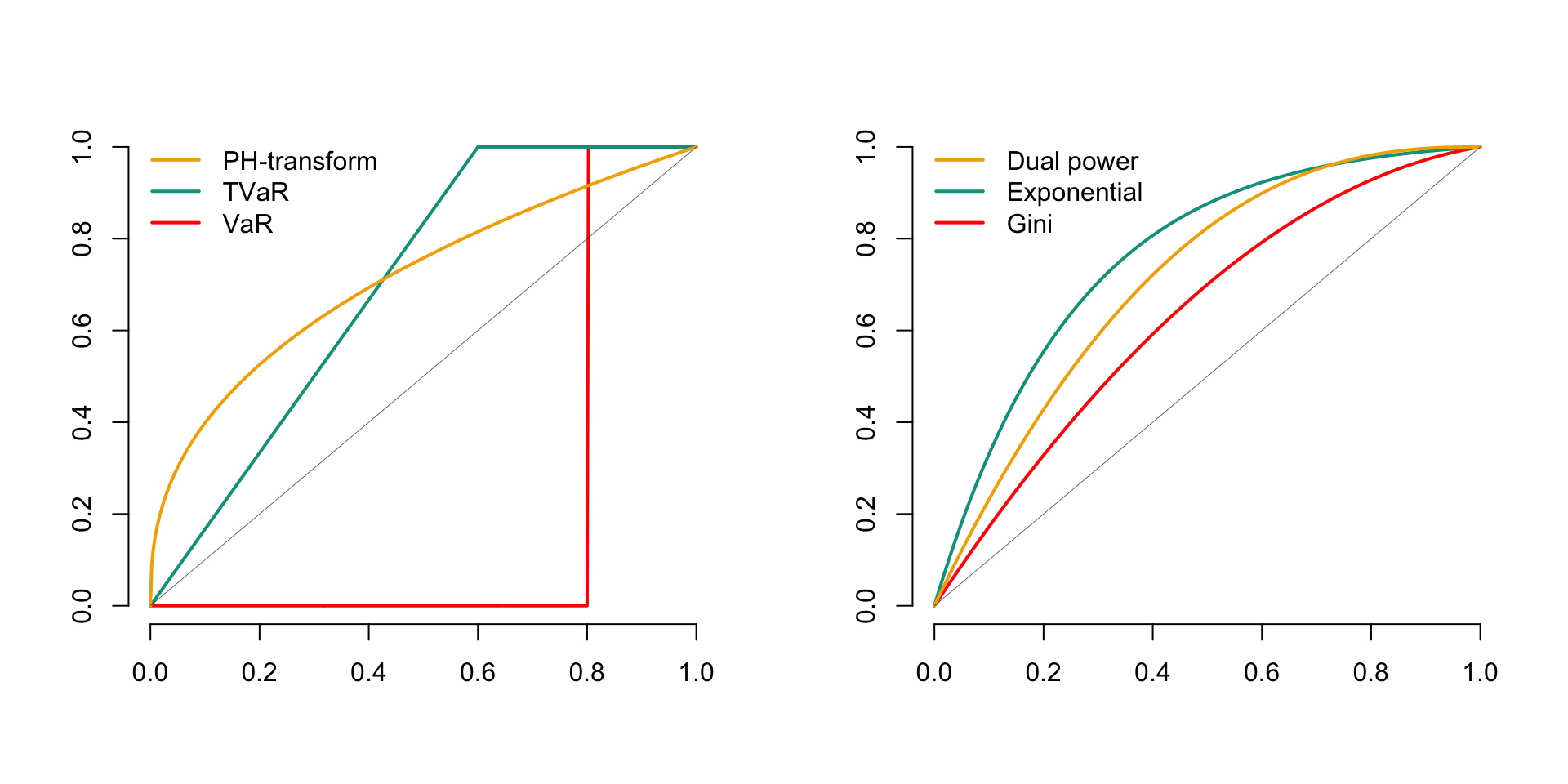
Figure 6.1: Major Distortion Functions
Remark. We will delve more deeply into different distortion functions in insurance microeconomics in Volume 2.
6.3 Main Properties of Wang’s Risk Measures
The main properties of Wang’s risk measures are summarized in the following result.
Proposition 6.3
- The risk measures of Wang are homogeneous.
- The risk measures of Wang are translation invariant.
- The risk measures of Wang are monotonic.
Proof. Working from Property 6.2, and considering the fact that VaR is translation invariant, we obtain \[\begin{eqnarray*} \rho _{g}\left[ X+c\right] &=&\int_{0}^{1}\text{VaR}[X+c;1-\alpha]\ dg(\alpha)\\ &=&\int_{0}^{1}\big(\text{VaR}[X;1-\alpha]+c\big)\ dg(\alpha)\\ &=&\rho_g[X]+c\big(g(1)-g(0)\big)=\rho_g[X]. \end{eqnarray*}\] This establishes (i). Similarly, we deduce the homogeneity and monotonicity of Wang’s measures from the corresponding properties of VaR.
6.3.1 Concavity of the Distortion Function
If the distortion function \(g\) is concave, the function \(x\mapsto g(\overline{F}_{X}(x))\) is right-continuous and is thus the tail function of a certain random variable. In this situation, \(\rho_{g}\left[ X\right]\) is indeed a mathematical expectation (not of \(X\) but of a variable \(Y\) with tail function \(\overline{F}_Y(y)=g(\overline{F}_{X}(y))\)). The following result illustrates the significance of the concavity assumption on \(g\).
When the distortion function is concave, the corresponding risk measure is subadditive.
6.4 Uniform Comparison of VaR
6.4.1 Definition
We have extensively studied the properties of VaR. Given two risks \(X\) and \(Y\), it is natural to compare them using the VaR corresponding to a level \(\alpha_1\), i.e., consider \(X\) to be less risky than \(Y\) if \(\text{VaR}[X;\alpha_1] \leq \text{VaR}[X;\alpha_1]\). However, often the choice of probability level is not immediately apparent, and it is possible to have simultaneously \[ \text{VaR}[X;\alpha_1] \leq \text{VaR}[X;\alpha_1] \] and \[ \text{VaR}[X;\alpha_2] \geq \text{VaR}[X;\alpha_2] \] for two probability levels \(\alpha_1\) and \(\alpha_2\). In such a situation, which of the risks, \(X\) or \(Y\), is less risky?
To avoid these difficulties, we will adopt the following definition, which suggests comparing the risks \(X\) and \(Y\) by requiring that the VaRs relative to these risks are ordered for any choice of the probability level.
Definition 6.10 Given two risks \(X\) and \(Y\), we will consider \(X\) less risky than \(Y\) based on VaR comparison, denoted as \(X\preceq_{\text{VaR}}Y\), when \[ \text{VaR}[X;\alpha] \leq \text{VaR}[Y;\alpha] \text{ for all } \alpha \in (0,1). \]
The relation \(\preceq_{\text{VaR}}\) that we have defined constitutes a partial order on the set of probability distributions (it can be easily verified to be reflexive, antisymmetric, and transitive). However, it is not antisymmetric with respect to random variables. Indeed, \(X\preceq_{\text{VaR}}Y\) and \(Y\preceq_{\text{VaR}}X\) do not imply \(X=Y\), but only \(X=_{\text{law}}Y\).
The relation \(\preceq_{\text{VaR}}\) has been studied extensively in probability and statistics (for example, see (Lehmann 1955)). It is better known in these fields as the stochastic order or distribution order. Economists and actuaries have also made significant use of it, under the name of first-order stochastic dominance. Other common notations for \(\preceq_{\text{VaR}}\) include \(\preceq_{st}\), \(\preceq_1\), or \(\preceq_{FSD}\).
6.4.2 Equivalent Conditions
We establish several equivalent conditions for having \(\preceq_{\text{VaR}}\) between two risks \(X\) and \(Y\). The first of these informs us that it is equivalent to compare VaRs or distribution functions (with the latter being the inverses of VaRs).
For two random variables \(X\) and \(Y\), \[\begin{eqnarray*} X\preceq_{\text{VaR}}Y &\Leftrightarrow& F_X(t)\geq F_Y(t) \text{ for all } t \in \mathbb{R},\\ &\Leftrightarrow& \overline{F}_X(t) \leq \overline{F}_Y(t) \text{ for all } t \in \mathbb{R}. \end{eqnarray*}\]
Interpreting \(\overline{F}_X(t)\) as the probability that \(X\) takes a “large” value (i.e., a value greater than \(t\)), this property shows that \(X\preceq_{\text{VaR}}Y\) means that \(X\) is “smaller” than \(Y\), since the probability that \(X\) takes large values is always less than that of \(Y\) taking large values.
Remark (Insensitivity of $\lst$ to Variance). The relation \(\preceq_{\text{VaR}}\) does not provide any information about the variances of the compared random variables. For example, if we take \(X\sim\text{Bernoulli}(p)\) and \(Y=1\), we have \(X\preceq_{\text{VaR}}Y\) even though \[ \text{Var}[X]=p(1-p)>\text{Var}[Y]=0. \] This demonstrates that \(\preceq_{\text{VaR}}\) focuses on comparing the magnitude of risks rather than their variability.
The stochastic order \(X\preceq_{\text{VaR}}Y\) allows us to derive numerous interesting inequalities, as demonstrated by the following result.
For two random variables \(X\) and \(Y\), \[ X\preceq_{\text{VaR}}Y \Leftrightarrow \mathbb{E}[g(X)] \leq \mathbb{E}[g(Y)] \text{ for all increasing functions } g, \] provided the expectations exist.
Proof. It suffices to recall that if \(U \sim \text{Uniform}(0,1)\), then \(X \stackrel{\text{d}}{=} \text{VaR}[X;U]\) according to Property ??. With this result in mind, we have the following representation, valid for any function \(g\): \[ \mathbb{E}[g(X)] = \mathbb{E}\left[g\left(\text{VaR}[X;U]\right)\right] = \int_0^1 g\left(\text{VaR}[X;u]\right)du. \] The stated result is then obtained simply by writing \[\begin{eqnarray*} \mathbb{E}[g(X)] &=& \int_0^1 g\left(\text{VaR}[X;u]\right)du \\ &\leq& \int_0^1 g\left(\text{VaR}[Y;u]\right)du = \mathbb{E}[g(Y)]. \end{eqnarray*}\]
In addition to the above results, we now demonstrate that we can restrict ourselves to regular functions \(g\) in Property ??.
Proposition 6.4 For two random variables \(X\) and \(Y\), \(X\preceq_{\text{VaR}}Y \Leftrightarrow \mathbb{E}[g(X)] \leq \mathbb{E}[g(Y)]\) for any function \(g\) such that \(g' \geq 0\), provided the expectations exist.
Proof. The implication ” \(\Rightarrow\) ” is evident. To prove the converse, note that \[ \mathbb{I}[x>t] = \lim_{\sigma\to 0}\Phi\left(\frac{x-t}{\sigma}\right). \] Furthermore, the function \(x \mapsto -\Phi\left(\frac{t-x}{\sigma}\right)\) is increasing. Therefore, we have in particular \[ -\mathbb{E}\left[\Phi\left(\frac{t-Y}{\sigma}\right)\right] \leq -\mathbb{E}\left[\Phi\left(\frac{t-X}{\sigma}\right)\right], \] which yields \[\begin{eqnarray*} \Pr[X>\text{Norm}(t,\sigma)] &=& \mathbb{E}\left[\Phi\left(\frac{X-t}{\sigma}\right)\right] \\ &\leq & \mathbb{E}\left[\Phi\left(\frac{Y-t}{\sigma}\right)\right] \\ &=& \Pr[Y>\text{Norm}(t,\sigma)] \end{eqnarray*}\] for any \(\sigma>0\). This same inequality holds when taking the limit as \(\sigma\to 0\), resulting in \(\Pr[X>t] \leq \Pr[Y>t]\). Since this reasoning holds for any \(t\), this concludes the proof.
6.4.2.1 Sufficient Conditions
Property ?? informs us that risks \(X\) and \(Y\) satisfy \(X\preceq_{\text{VaR}}Y\) when their respective tail functions mutually dominate each other. The following result provides a sufficient condition for this to hold. It suffices that the probability density functions only cross once.
Proposition 6.5 For any risks \(X\) and \(Y\), if \(f_X(t) \geq f_Y(t)\) for \(t<c\) and \(f_X(t) \leq f_Y(t)\) for \(t>c\), then \(X\preceq_{\text{VaR}}Y\).
Proof. It suffices to observe that if \(x<c\), \[ F_X(x) = \int_0^x f_X(t)dt \geq \int_0^x f_Y(t)dt = F_Y(x) \] and if \(x>c\), \[ \overline{F}_X(x) = \int_x^{+\infty} f_X(t)dt \geq \int_x^{+\infty} f_Y(t)dt = \overline{F}_Y(x). \] Thus, we have \(X\preceq_{\text{VaR}}Y\) under the conditions stated above, which completes the proof.
6.4.3 Properties
6.4.3.1 Stability of \(\preceq_{\text{VaR}}\) with respect to standard deductible clauses
The developments in this paragraph are based on the following result.
Proposition 6.6 For any random variables \(X\) and \(Y\), \[ X\preceq_{\text{VaR}}Y \Rightarrow t(X)\preceq_{\text{VaR}}t(Y) \] for any non-decreasing function \(t\).
Proof. The result is immediately deduced from the following observation: for any non-decreasing function \(g\), the function \(x\mapsto g(t(x))\) is non-decreasing when \(t\) is non-decreasing.
Property 6.6 guarantees, among other things, that when \(X\preceq_{\text{VaR}}Y\), \[\begin{eqnarray*} (X-\delta)_+ & \preceq_{\text{VaR}}&(Y-\delta)_+\text{ for any deductible }\delta\in{\mathbb{R}},\\ &&\text{mandatory underwriting,}\\ \alpha X & \preceq_{\text{VaR}}&\alpha Y\text{ for any }\alpha>0,\\ X\mathbb{I}[X>\kappa] & \preceq_{\text{VaR}}&Y\mathbb{I}[Y>\kappa]\text{ for any threshold }\kappa\in{\mathbb{R}},\\ \min\{X,\omega\} & \preceq_{\text{VaR}}&\min\{Y,\omega\}\text{ for any cap }\omega\in{\mathbb{R}}. \end{eqnarray*}\] This implies that a comparison in the \(\preceq_{\text{VaR}}\) sense is not affected by the introduction of a standard deductible clause related to damages (whether it’s a mandatory underwriting, a deductible, or an upper limit) in the policy terms.
6.4.3.2 Stability of \(\preceq_{\text{VaR}}\) in the Presence of Uncertainty
Regardless of the risks \(X\) and \(Y\) and the random vector \(\boldsymbol{\Theta}\), if \(X\preceq_{\text{VaR}}Y\) when \(\boldsymbol{\Theta}=\boldsymbol{\theta}\), then the stochastic inequality remains valid when \(\boldsymbol{\Theta}\) is unknown. Indeed, as \[ \Pr[X\leq x|\boldsymbol{\Theta}=\boldsymbol{\theta}]\geq \Pr[Y\leq x|\boldsymbol{\Theta}=\boldsymbol{\theta}] \text{ for all }\boldsymbol{\theta}\text{ and }x, \] we easily deduce that \[\begin{eqnarray*} \Pr[X\leq x] & = & \int_{\boldsymbol{\theta}}\Pr[X\leq x|\boldsymbol{\Theta}=\boldsymbol{\theta}] dF_{\boldsymbol{\Theta}}(\boldsymbol{\theta})\\ & \geq & \int_{\boldsymbol{\theta}} \Pr[Y\leq x|\boldsymbol{\Theta}=\boldsymbol{\theta}] dF_{\boldsymbol{\Theta}}(\boldsymbol{\theta})=\Pr[Y\leq x], \end{eqnarray*}\] which proves the announced result.
6.4.4 Hazard Rate and PH Risk Measure
6.4.4.1 Definition and Equivalent Conditions
We could be interested in comparing risks given that they exceed a certain level \(t\). Thus, we could require that \[ [X|X>t]\preceq_{\text{VaR}}[Y|Y>t] \] for any level \(t\). The following example shows that this is not necessarily true when \(X\preceq_{\text{VaR}}Y\).
Example 6.3 Show that \[\begin{equation*} X\preceq_{\text{VaR}}Y\nRightarrow [X|X>t] \preceq_{\text{VaR}}[Y|Y>t] \text{ for any }t. \end{equation*}\] Consider, for instance, the case where \(X\sim \mathcal{U}ni(0,3)\) and \(Y\) has the density \[ f_{Y}\left( x\right) =\frac{1}{6} \mathbb{I}_{\left] 0,1\right] }\left( x\right)+\frac{1}{2}\mathbb{I}_{\left] 1,2\right] }\left( x\right)+ \frac{1}{3}\mathbb{I}_{\left] 2,3\right[ }\left(x\right). \] Then, \(X\preceq_{\text{VaR}}Y\), but \([X|X>1]\sim\mathcal{U}ni(1,3)\) and \([Y|Y>1]\) has the density \[ f_{Y}^{\ast }\left( x\right) =\frac{3}{5}\mathbb{I}_{\left] 1,2\right] }\left( x\right)+\frac{2}{5}\mathbb{I}_{\left] 2,3\right[ }\left(x\right) \] so that \[ [Y|Y>1]\preceq_{\text{VaR}}[X|X>1]. \]
We can prove the following result.
Proposition 6.7 Given two risks \(X\) and \(Y\), \([X|X>t]\preceq_{\text{VaR}}[Y|Y>t]\) for any \(t\in{\mathbb{R}}\) if, and only if \[\begin{eqnarray*} &\Leftrightarrow & t\mapsto \frac{\overline{F}_Y(t)}{\overline{F}_X(t)}\text{ is non-decreasing}(\#eq:eq1.B.3b)\\ &\Leftrightarrow & \overline{F}_X(u)\overline{F}_Y(v)\ge\overline{F}_X(v)\overline{F}_Y(u)\quad \text{for any}\quad u\le v.(\#eq:eq1.B.4) \end{eqnarray*}\]
This comparison can be related to the hazard rates, as shown in the following result.
Given two risks \(X\) and \(Y\), \([X|X>t]\preceq_{\text{VaR}}[Y|Y>t]\) for any \(t\in{\mathbb{R}}\) if, and only if \(r_X(t)\geq r_Y(t)\) for any \(t\).
Proof. The ratio \(\overline{F}_Y/\overline{F}_X\) is non-decreasing if, and only if, \(\ln \overline{F}_Y/\overline{F}_X\) is also non-decreasing. This further implies that \(\ln \overline{F}_Y-\ln\overline{F}_X\) is non-decreasing, which is equivalent to \(r_X-r_Y>0\) since, according to Property ??, \[ \frac{d}{dt}\Big\{\ln\overline{F}_Y(t)-\ln\overline{F}_X(t)\Big\}=r_X(t)-r_Y(t). \]
6.4.4.2 Hazard Rate and PH Risk Measure
Let’s suppose we deflate the hazard rate by a factor \(\xi\), i.e., we transition from a rate \(r_X\) to a rate \(r_{X^*}\) given by \[ r_{X^*}(t)=\frac{r_X(t)}{\xi}\leq r_X(t),\text{ for }\xi\geq 1. \] Using Property ??, we obtain a tail function \[ \overline{F}_{X^*}(t)=\exp\left(-\int_0^t\frac{r_X(s)}{\xi}ds\right)=\{\overline{F}_X(t)\}^{1/\xi}. \] Therefore, PH\([X;\xi]=\mathbb{E}[X^*]\). The PH risk measure consists of replacing the original risk \(X\) with a transformed risk \(X^*\) whose hazard rate has been deflated, and then calculating the expectation associated with \(X^*\). We have \[ [X|X>t]\preceq_{\text{VaR}}[X^*|X^*>t]\text{ for any }t>0. \]
6.4.5 Likelihood Ratio and Esscher Principle
6.4.5.1 Definition
We could also consider imposing \[ [X|a\leq X\leq a+h]\preceq_{\text{VaR}}[Y|a\leq Y\leq a+h] \] for any level \(a\) and increment \(h>0\). This corresponds to the situation of a reinsurer who would cover the interval \((a,a+h]\) of a risk \(X\), i.e., who would expose themselves to a loss of \[ X_{(a,a+h]}= \left\{ \begin{array}{l} 0\text{ if }X<a\\ X-a\text{ if }a\leq X<a+h\\ h\text{ if }a+h\leq X, \end{array} \right. \] where \(a\) is the retention and \(h\) is the limit.
We can establish the following result.
(#prp:Propo5.4.10) Consider the random variables \(X\) and \(Y\), both continuous or discrete, with probability density functions \(f_X\) and \(f_Y\). If \[\begin{equation} \frac{f_X(t)}{f_Y(t)}\quad\text{decreases over the union of the supports of $X$ and $Y$} (\#eq:eq1.C.1) \end{equation}\] (taking \(a/0\) as \(+\infty\) when \(a>0\) by convention), or equivalently, if \[\begin{equation} f_X(u)f_Y(v)\ge f_X(v)f_Y(u)\quad\text{for all}\quad u\le v, (\#eq:eq1.C.2) \end{equation}\] then \([X|a\leq X\leq a+h]\preceq_{\text{VaR}}[Y|a\leq Y\leq a+h]\) for any level \(a\) and increment \(h>0\).
Proof. Consider \(a<b\). The stochastic inequality \([X|a\leq X\leq b]\preceq_{\text{VaR}}[Y|a\leq Y\leq b]\) guarantees that \[ \frac{\Pr[u\le X\le b]}{\Pr[a\le X\le b]}\le\frac{\Pr[u\le Y\le b]} {\Pr[a\le Y\le b]}\quad\text{when}\quad u\in[a,b]. \] This implies \[ \frac{\Pr[a\le X<u]}{\Pr[u\le X\le b]}\ge\frac{\Pr[a\le Y<u]} {\Pr[u\le Y\le b]}\quad\text{when}\quad u\in [a,b]. \] In other words, \[ \frac{\Pr[a\le X<u]}{\Pr[a\le Y<u]}\ge\frac{\Pr[u\le X\le b]} {\Pr[u\le Y\le b]}\quad\text{when}\quad u\in [a,b]. \] Particularly, for \(u<b\le v\), \[ \frac{\Pr[u\le X<b]}{\Pr[u\le Y<b]}\ge\frac{\Pr[b\le X\le v]} {\Pr[b\le Y\le v]}. \] Hence, when \(X\) and \(Y\) are continuous, \[ \frac{\Pr[a\le X<u]}{\Pr[a\le Y<u]}\ge\frac{\Pr[b\le X\le v]} {\Pr[b\le Y\le v]}\quad\text{when}\quad a<u\le b\le v. \] Taking limits as \(a\rightarrow u\) and \(b\rightarrow v\), we obtain @ref(eq:eq1.C.2). The proof in the discrete case is similar.
The conditions @ref(eq:eq1.C.1) and @ref(eq:eq1.C.2), seemingly technical and not very intuitive, are generally easy to establish in parametric models.
Remark. The method of comparing probability distributions discussed in Proposition @ref(prp:Propo5.4.10) is also called the likelihood ratio order and denoted by \(\preceq_{lr}\).
6.4.5.2 Connection with the Esscher Transform
Let \(X_h\) be the Esscher transform of \(X\). The ratio of the probability densities associated with \(X\) and \(X_h\) is proportional to \(\exp(-hx)\), which is clearly decreasing in \(x\). This indicates that \[ [X|a\leq X\leq b]\preceq_{\text{VaR}}[X_h|a\leq X_h\leq b], \] for any \(a<b\).
The following result shows under which conditions the Esscher risk measures relative to two risks \(X\) and \(Y\) are uniformly ordered.
Proposition 6.8 If \([X|a\leq X\leq b]\preceq_{\text{VaR}}[Y|a\leq Y\leq b]\) for any \(a<b\), then \({\text{Es}}[X;h]\leq{\text{Es}}[Y;h]\) for any \(h>0\).
Proof. Due to Proposition @ref(prp:Propo5.4.10), we know that the inequality \[ f_X(u)f_Y(v)\geq f_X(v)f_Y(u) \] holds for any \(u\leq v\). By multiplying both sides of this inequality by \[ \frac{\exp(hu)}{M_X(h)} \frac{\exp(hv)}{M_Y(h)} \] we obtain the same inequality for the probability density functions of \(X_h\) and \(Y_h\), from which we conclude that \([X_h|a\leq X_h\leq b]\preceq_{\text{VaR}}[Y_h|a\leq Y_h\leq b]\), giving the desired result.
6.5 Uniform Comparison of TVaRs
6.5.1 Definition
Here, we introduce a new method of comparing risks based on Tail Value-at-Risk (TVaR).
Definition 6.11 For any random variables \(X\) and \(Y\) with finite mean, \(X\) will be considered less risky than \(Y\) based on the comparison of TVaRs, denoted as \(X\preceq_{\text{TVaR}}Y\), when \[ {\text{TVaR}}[X;\alpha]\leq{\text{TVaR}}[Y;\alpha]\text{ for all }\alpha\in[0,1]. \]
The restriction to risks with finite mean ensures the existence of TVaRs, and thus the correctness of the definition of \(\preceq_{\text{TVaR}}\). Therefore, we now only compare risks with finite pure premium (it’s worth noting that many results we will establish in the following section depend on this assumption). This distinction also sets apart \(\preceq_{\text{VaR}}\) and \(\preceq_{\text{TVaR}}\): indeed, \(\preceq_{\text{VaR}}\) is defined for any variables in consideration, whereas this is not the case for \(\preceq_{\text{TVaR}}\).
The \(\preceq_{\text{TVaR}}\) relation is quite old (it’s a direct descendant of the relation known as “majorization” among numerical vectors, studied in the 1930s). Actuaries still refer to it as the stop-loss order (denoted \(\preceq_{sl}\)), a concept closely related to the second-order stochastic dominance (often denoted as \(\preceq_2\) or \(\preceq_{SSD}\)) in economics. Probability theorists are more familiar with the \(\preceq_{\text{TVaR}}\) relation under the name of increasing convex order (denoted \(\preceq_{icx}\)).
We will also use the relation denoted \(\preceq_{\text{TVaR,=}}\), which restricts \(\preceq_{\text{TVaR}}\) to pairs of random variables with the same mean.
Definition 6.12 For any random variables \(X\) and \(Y\), \[\begin{eqnarray*} X\preceq_{\text{TVaR,=}}Y&\Leftrightarrow& \left\{ \begin{array}{l} \mathbb{E}[X]=\mathbb{E}[Y],\\ X\preceq_{\text{TVaR}}Y, \end{array} \right. \\ &\Leftrightarrow& \left\{ \begin{array}{l} {\text{TVaR}}[X;0]={\text{TVaR}}[Y;0],\\ {\text{TVaR}}[X;\alpha]\leq{\text{TVaR}}[Y;\alpha]\\ \hspace{20mm}\text{for all }\alpha\in(0,1). \end{array} \right. \end{eqnarray*}\]
The \(\preceq_{\text{TVaR,=}}\) relation is known as the convex order among probability theorists (denoted \(\preceq_{cx}\)). It is closely related to other relations, such as the Lorenz order.
Remark. Note that \(\preceq_{\text{VaR}}\) did not allow the comparison of random variables with the same mean. Indeed, for any risks \(X\) and \(Y\), \[ \left. \begin{array}{l} X\preceq_{\text{VaR}}Y\\ \mathbb{E}[X]=\mathbb{E}[Y] \end{array} \right\} \Rightarrow X=_{\text{law}} Y. \] To prove this result, it suffices to examine the identity \[ \mathbb{E}[Y]-\mathbb{E}[X]=\int_{x=0}^{+\infty} \underbrace{\{\Pr[Y>x]-\Pr[X>x]\}}_{\geq 0 \text{ for all }x}dx=0, \] which implies \(\Pr[Y>x]=\Pr[X>x]\) for all \(x\) and concludes the verification.
6.5.2 Equivalent Conditions
6.5.2.1 Tail-VaR and Stop-Loss Premiums
The \(\preceq_{\text{TVaR}}\) and \(\preceq_{\text{TVaR,=}}\) relations introduced above can also be characterized using stop-loss premiums, as shown by the following result.
Proposition 6.9
- For given two risks \(X\) and \(Y\), \[ X\preceq_{\text{TVaR}}Y\Leftrightarrow\mathbb{E}[(X-t)_+]\leq \mathbb{E}[(Y-t)_+] \text{ for all } t \in {\mathbb{R}}. \]
- For given two risks \(X\) and \(Y\) with the same finite mean \(\mu\), \[ X\preceq_{\text{TVaR,=}}Y\Leftrightarrow\mathbb{E}[(X-t)_+]\leq \mathbb{E}[(Y-t)_+] \text{ for all } t \in {\mathbb{R}}. \]
Proof. We only prove (i); the reasoning for (ii) is similar. First, assume that the stop-loss premiums for \(X\) and \(Y\) are ordered for any \(t\), and consider the function \[\begin{eqnarray*} h(t)&=&(1-\alpha)t+\mathbb{E}[(X-t)_+]\\ &=&(1-\alpha)t+\int_t^{+\infty}\overline{F}_X(x)dx \end{eqnarray*}\] for fixed \(0<\alpha<1\). As \[ \overline{F}_X\Big({\text{VaR}}[X;\alpha]\Big)\leq 1-\alpha\leq \Pr\Big[X\geq {\text{VaR}}[X;\alpha]\Big], \] the function \(h\) achieves its minimum at \(t={\text{VaR}}[X;\alpha]\), and the same holds for the function \(\frac{h(t)}{1-\alpha}\). This allows us to write using (6.2), \[\begin{eqnarray*} {\text{TVaR}}[X;\alpha]&=&{\text{VaR}}[X;\alpha]+\frac{1}{1-\alpha}{\text{ES}}[X;\alpha]\\ &=&\frac{h\Big({\text{VaR}}[X;\alpha]\Big)}{1-\alpha}\\ &\leq &\frac{h\Big({\text{VaR}}[Y;\alpha]\Big)}{1-\alpha}\\ &=&{\text{VaR}}[Y;\alpha]+\frac{1}{1-\alpha}\mathbb{E}\Big[\Big(X-{\text{VaR}}[Y;\alpha]\Big)_+\Big]\\ &\leq&{\text{VaR}}[Y;\alpha]+\frac{1}{1-\alpha}\mathbb{E}\Big[\Big(Y-{\text{VaR}}[Y;\alpha]\Big)_+\Big]\\ &=&{\text{TVaR}}[Y;\alpha]. \end{eqnarray*}\] Therefore, the TVaRs for \(X\) and \(Y\) are ordered for any probability level \(\alpha\).
Conversely, assume that the TVaRs are ordered, and show that then the stop-loss premiums must also be ordered. We saw in exercise @ref(eq:ExoSL} that \[ \mathbb{E}[(X-t)_+]=\int_{\alpha=F_X(t)}^1{\text{VaR}}[X;\alpha]d\alpha-t\overline{F}_X(t), \] then for \(t\) such that \(0<F_X(t)<1\), \[\begin{eqnarray*} \mathbb{E}[(X-t)_+]&=&\overline{F}_X(t)\Big\{{\text{TVaR}}\big[X;F_X(t)\big]-t\Big\}\\ &\leq&\overline{F}_X(t)\Big\{{\text{TVaR}}\big[Y;F_X(t)\big]-t\Big\}\\ &=&\int_{\alpha=F_X(t)}^1{\text{VaR}}[Y;\alpha]d\alpha-t\overline{F}_X(t)\\ &=&\int_{\alpha=F_Y(t)}^1{\text{VaR}}[Y;\alpha]d\alpha-t\overline{F}_Y(t)\\ &&+\int_{\alpha=F_X(t)}^{F_Y(t)}{\text{VaR}}[Y;\alpha]d\alpha-t\Big(F_Y(t)-F_X(t)\Big)\\ &=&\mathbb{E}[(Y-t)_+]+\int_{\alpha=F_X(t)}^{F_Y(t)}\Big({\text{VaR}}[Y;\alpha]-t\Big)d\alpha. \end{eqnarray*}\] As \(\alpha\leq F_Y(t)\Leftrightarrow t\geq{\text{VaR}}[Y;\alpha]\), the second term is negative, which guarantees that \(\mathbb{E}[(X-t)_+]\leq \mathbb{E}[(Y-t)_+]\), concluding the proof. \end{proof}
We now know that the \(\preceq_{\text{TVaR,=}}\) and \(\preceq_{\text{TVaR}}\) relations can be interpreted using reinsurance premiums relative to a stop-loss treaty. A comparison in the \(\preceq_{\text{TVaR}}\) or \(\preceq_{\text{TVaR,=}}\) sense boils down to comparing stop-loss premiums for different retentions. Therefore, when it comes to choosing between two risks \(X\) and \(Y\), reinsurers are consulted: they are asked about their pure stop-loss rates, and preference is given to the risk for which reinsurance premiums are always more advantageous, while keeping the mean constant.
6.5.2.2 Tail-VaR and Convex Functions
Similar to \(\preceq_{\text{VaR}}\) being linked to increasing functions, the \(\preceq_{\text{TVaR,=}}\) and \(\preceq_{\text{TVaR}}\) relations are related to convex and convex increasing functions, as shown by the following results.
Proposition 6.10 For any two random variables \(X\) and \(Y\) with finite means, we have
- \(X\preceq_{\text{TVaR,=}}Y\Leftrightarrow \mathbb{E}[g(X)]\leq\mathbb{E}[g(Y)]\) for any convex function \(g\), provided the expectations exist.
- \(X\preceq_{\text{TVaR,=}}Y\Leftrightarrow \mathbb{E}[g(X)]\leq\mathbb{E}[g(Y)]\) for any function \(g\) such that \(g''\geq 0\), provided the expectations exist.
Proof. Let’s prove (i). The implication ” \(\Leftarrow\) ” is evident since the function \(x\mapsto(x-t)_+\) is convex for any \(t\in {\mathbb{R}}^+\). To prove ” \(\Rightarrow\) “, proceed as follows. Any convex function \(g\) can be approximated uniformly by a sequence \(\{g_n,\hspace{2mm}n=1,2,\ldots\}\) of convex functions defined by \[ g_n(x)=\alpha_1^{(n)}+\alpha_2^{(n)} x+\sum_{j=0}^n\beta_j^{(n)}(x-t_j^{(n)})_+, \] where \(\alpha_1^{(n)},\alpha_2^{(n)}\in {\mathbb{R}}\), \(\beta_j^{(n)}\geq 0\) for \(j=0,1,\ldots,n\), and \(0<t_0^{(n)}<t_1^{(n)}<\ldots<t_n^{(n)}\). Thus, as the inequality \[\begin{eqnarray*} \mathbb{E}[g_n(X)] & = & \alpha_1^{(n)}+\alpha_2^{(n)} \mathbb{E}[X]+\sum_{j=0}^n\beta_j^{(n)} \mathbb{E}[(X-t_j^{(n)})_+] \\ & \leq & \alpha_1^{(n)}+\alpha_2^{(n)} \mathbb{E}[X]+\sum_{j=0}^n\beta_j^{(n)} \mathbb{E}[(Y-t_j^{(n)})_+]=\mathbb{E}[g_n(Y)] \end{eqnarray*}\] is satisfied for any \(n\), it follows that \(\mathbb{E}[g(X)]\leq \mathbb{E}[g(Y)]\) when passing to the limit, which completes the proof of (i). The proof of (ii) is similar to that of Property ??.
Remark (Variability). Roughly speaking, convex functions are those that attain their highest values in regions of the form \(]-\infty ,a[ \cup ]b, +\infty[\), where \(a<b\). For this reason, if \(X\preceq_{\text{TVaR,=}}Y\), \(Y\) takes on values that are more “extreme” than those of \(X\), meaning that \(Y\) is more “variable” than \(X\). This can also be justified by the fact that if \(X\preceq_{\text{TVaR,=}}Y\), then necessarily \[ \mathbb{V}[X]\leq \mathbb{V}[Y]; \] this stems from the fact that the function \(x\mapsto g(x)=x^2\) is convex.
By proceeding similarly, we can establish the following result.
Proposition 6.11 For any two random variables \(X\) and \(Y\) with finite means, we have
- \(X\preceq_{\text{TVaR}}Y\Leftrightarrow \mathbb{E}[g(X)]\leq\mathbb{E}[g(Y)]\) for any convex increasing function \(g\), provided the expectations exist.
- \(X\preceq_{\text{TVaR}}Y\Leftrightarrow \mathbb{E}[g(X)]\leq\mathbb{E}[g(Y)]\) for any function \(g\) such that \(g'\geq 0\) and \(g"\geq 0\), provided the expectations exist.
6.5.2.3 Strassen’s Characterization
The following characterization was obtained by Strassen in 1965. It shows that Tail-VaR is decreased by taking conditional expectations.
Proposition 6.12 For given two risks \(X\) and \(Y\), \(X\preceq_{\text{TVaR,=}}Y\) if and only if we can find two random variables \(\widetilde{X}\) and \(\widetilde{Y}\) (defined on the same probability space) such that \(\widetilde{X}=_{\text{law}}X\), \(\widetilde{Y}=_{\text{law}}Y\), and \(\mathbb{E}[\widetilde{Y}|\widetilde{X}]=\widetilde{X}\).
Proof. Constructing the variables \(\widetilde{X}\) and \(\widetilde{Y}\) (i.e., proving the necessity of Strassen’s condition) is challenging; we refer interested readers to (Müller and Stoyan 2002) for an interesting proof. The sufficiency is easy to establish. Indeed, if such variables \(\widetilde{X}\) and \(\widetilde{Y}\) exist, then for any convex function \(g\), \[\begin{eqnarray*} \mathbb{E}[g(X)] & = & \mathbb{E}[g(\widetilde{X})]=\mathbb{E} \Big[g\Big(\mathbb{E}[\widetilde{Y}|\widetilde{X}]\Big)\Big] \\ & \leq & \mathbb{E}\Big[\Big(\mathbb{E}[g(\widetilde{Y})|\widetilde{X}]\Big)\Big] =\mathbb{E}[g(\widetilde{Y})]=\mathbb{E}[g(Y)] \end{eqnarray*}\] by virtue of Jensen’s inequality.
Corollary 6.2 In particular, overlaying an additional centered randomness \(\epsilon\) onto a risk \(X\) makes the situation riskier (in fact, more variable). Formally, for any risk \(X\) and a random variable \(\epsilon\) independent of \(X\) with \(\mathbb{E}[\epsilon]=0\), \[ X\preceq_{\text{TVaR,=}}X+\epsilon. \]
6.5.3 Sufficient Condition
We provide sufficient conditions for \(\preceq_{\text{TVaR,=}}\) and \(\preceq_{\text{TVaR}}\) based on the number of crossings of cumulative distribution functions.
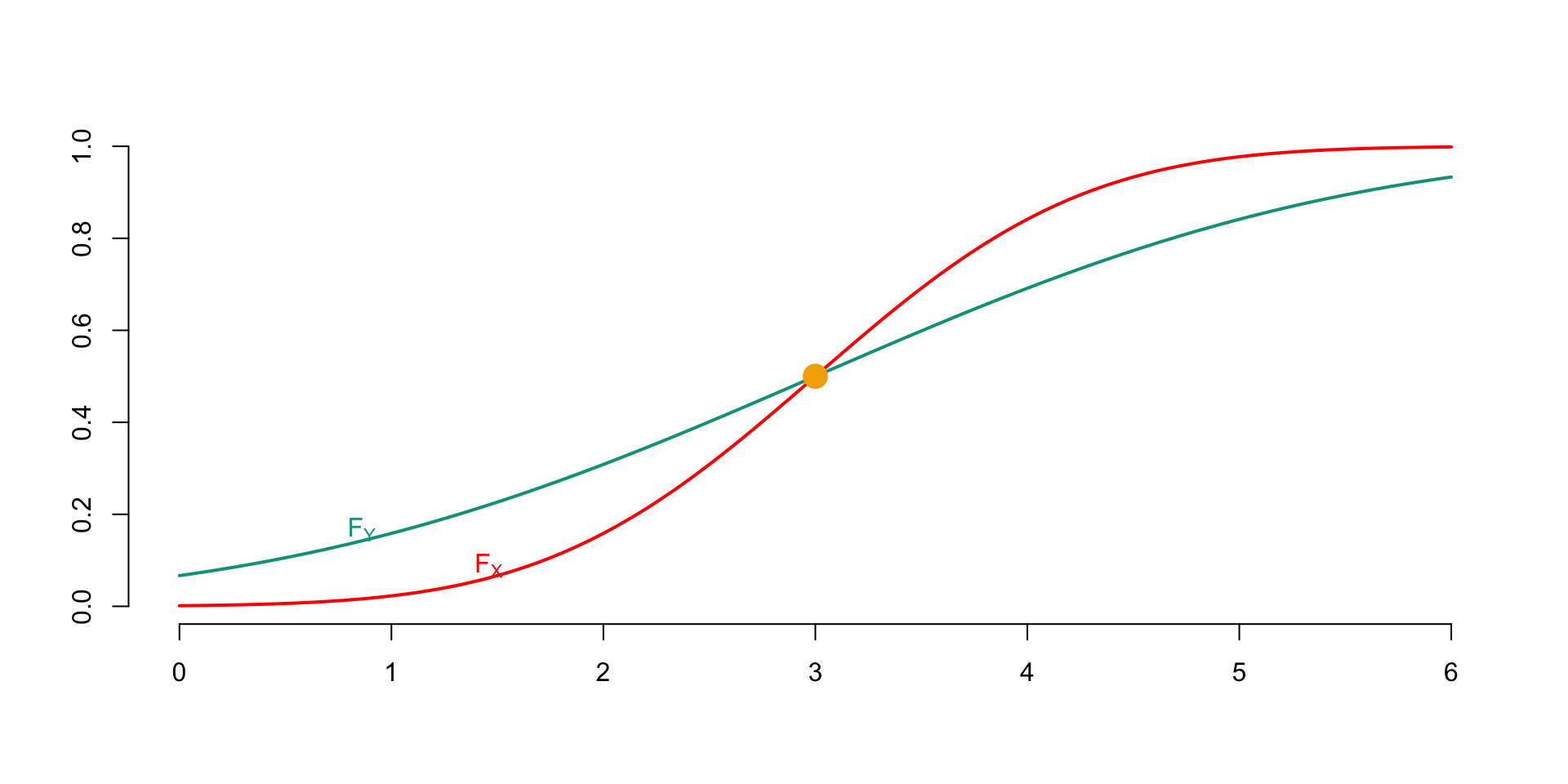
Figure 6.2: Two cumulative distribution functions \(F_X\) and \(F_Y\) satisfying the single crossing property
(#prp:p2.c.2) Let \(X\) and \(Y\) be two random variables such that \(\mathbb{E}[X]=\mathbb{E}[Y]\). If there exists a constant \(c\) such that \[ F_Y(x)\geq F_X(x)\text{ for all } x<c, \] and \[ F_Y(x)\leq F_X(x) \text{ for all } x>c, \] then \(X\preceq_{\text{TVaR,=}}Y\).
Proof. For \(t>c\), we have \[\begin{eqnarray*} \mathbb{E}[(X-t)_+] & = & \int_{x=t}^{+\infty}\Pr[X>x]dx\\ & \leq & \int_{x=t}^{+\infty}\Pr[Y>x]dx\\ & = & \mathbb{E}[(Y-t)_+]. \end{eqnarray*}\] For \(t\leq c\), it suffices to note that \[\begin{eqnarray*} \mathbb{E}[(X-t)_+]&=&\mathbb{E}[X]-\int_{x=0}^{t}\Pr[X>x]dx\\ &=&\mathbb{E}[X]-\int_{x=0}^{t}\Pr[Y>x]dx, \end{eqnarray*}\] which yields the result as \(\mathbb{E}[X]=\mathbb{E}[Y]\).
Similarly, we can prove the following result.
(#prp:2.c.2) Let \(X\) and \(Y\) be two random variables such that \(\mathbb{E}[X]\leq\mathbb{E}[Y]\). If there exists a constant \(c\) such that \[ F_Y(x)\geq F_X(x)\text{ for all } x<c, \] and \[ F_Y(x)\leq F_X(x) \text{ for all } x>c, \] then \(X\preceq_{\text{TVaR}}Y\).
6.5.4 Properties
6.5.4.1 Revisited Law of Large Numbers
We reexamine the law of large numbers here. Specifically, we show that there is actually a decreasing sense of \(\preceq_{\text{TVaR,=}}\) for the arithmetic means as \(n\) increases.
Proposition 6.13 For independent and identically distributed risks \(X_1,X_2,X_3,\ldots\) with the same finite mean, we denote \[ \overline{X}^{(n)}=\frac{1}{n}\sum_{i=1}^n X_i. \] We then have \[ \overline{X}^{(n+1)}\preceq_{\text{TVaR,=}}\overline{X}^{(n)}. \]
Proof. It suffices to observe that \[ \mathbb{E}\big[X_i\big|\overline{X}^{(n)}\big]=\overline{X}^{(n)} \] for any \(i=1,\ldots,n\). Thus, \[ \mathbb{E}\big[\overline{X}^{(n-1)}\big|\overline{X}^{(n)}\big]=\overline{X}^{(n)}, \] which gives the result using Proposition 6.12.
It’s worth mentioning that this gives an interesting interpretation of the law of large numbers. Indeed, the convergence of \(\overline{X}^{(n)}\) to \(\mathbb{E}[X_1]\) is accompanied by a monotonic reduction of risk (as measured by Tail-VaR). Furthermore, for any \(n\), \[ \mathbb{E}[X_1]\preceq_{\text{TVaR,=}}\overline{X}^{(n)}. \]
This result also illustrates the reduction in variability resulting from pooling an increasing number of identical risks. The stability of the company’s outcome will be even greater when the number of risks in the portfolio is large.
6.5.4.2 Advantages of Policy Standardization
On the market, it’s noticeable that policy conditions are standardized. Even though the individual situations of insured parties are all different, insurers refuse to take this into account and organize the transfer of risks under similar conditions for all insured parties. They only personalize certain risk features in specific conditions. One could legitimately question the relevance of this practice: beyond the administrative management simplification benefits, is it always appropriate to treat insured parties identically? The following result provides an answer to this question.
Proposition 6.14 For independent and identically distributed risks \(X_1,X_2,X_3,\ldots\), regardless of the functions \(g_1, g_2, g_3,\ldots\),
\[
\sum_{i=1}^{n} \overline{g}(X_i)\preceq_{\text{TVaR,=}}\sum_{i=1}^n
g_i(X_i)\text{ where }
\overline{g}(x)=\frac{1}{n} \sum_{i=1}^n g_i(x).
\]
Proof. Let \(\pi=\{\pi(1),\pi(2),\ldots,\pi(n)\}\) be a random permutation of \(\{1,2,\ldots,n\}\), independent of the \(X_i\). Let \(\mathcal{P}\) be the set of such permutations. Then, \[\begin{eqnarray*} &&\mathbb{E}\left[\left.\sum_{i=1}^ng_{\pi(i)}(X_i)\right| X_1,X_2,\ldots,X_n\right] \\ & = & \frac{1}{n!}\sum_{\{\xi_1,\ldots,\xi_n\}\in\cal P} \left\{g_{\xi_1}(X_1)+g_{\xi_2}(X_2)+\ldots +g_{\xi_n}(X_n)\right\} \\ \\ & = & \sum_{i=1}^n{\bar g}(X_i), \end{eqnarray*}\] which implies \[\begin{eqnarray*} &&\mathbb{E}\left[\left.\sum_{i=1}^ng_{\pi(i)}(X_i)\right| \sum_{i=1}^n{\bar g}(X_i)\right] \\ & = & \mathbb{E}\left[\mathbb{E}\left[\left.\sum_{i=1}^ng_{\pi(i)}(X_i)\right| X_1,X_2,\ldots,X_n\right]\left| \sum_{i=1}^n{\bar g}(X_i)\right.\right] \\ \\ & = & \sum_{i=1}^n{\bar g}(X_i). \end{eqnarray*}\] Then, using Strassen’s characterization, we can state that \[\begin{equation} \sum_{i=1}^n{\bar g}(X_i)\preceq_{\text{TVaR,=}}\sum_{i=1}^ng_{\pi(i)}(X_i). (\#eq:eq1.4) \end{equation}\] Finally, the result follows from @ref(eq:eq1.4) since \(\sum_{i=1}^ng_{\pi(i)}(X_i)\) and \(\sum_{i=1}^ng_i(X_i)\) are identically distributed.
This result explains why insurance contracts are standardized (in addition to the management facilitation benefits, of course). Indeed, if the actuary has to manage \(n\) identical risks resulting in annual costs \(X_1,X_2,\ldots,X_n\), they always have an interest in applying the same treatment to these risks.
Example 6.4 For example, if the insurer decides to leave a percentage of the claim amount to the insured, this percentage must be the same for all insured parties in the same category. Indeed, if the insurer leaves \(\alpha_i\%\) of the claims at the expense of insured party number \(i\), their situation will always be worse than that of the insurer who leaves \(\overline{\alpha}\%\) of the claims at the expense of each insured party, where \[ \overline{\alpha}=\frac{1}{n}\sum_{i=1}^n\alpha_i \] since \[ \sum_{i=1}^n\overline{\alpha}X_i\preceq_{\text{TVaR,=}}\sum_{i=1}^n\alpha_iX_i. \]
To increase the stability of the company’s outcomes, the actuary will always have an interest in applying the same treatment to all identical policies in their portfolio.
6.5.4.3 Stability of Preferences
For any risks \(X\) and \(Y\) such that \(X\preceq_{\text{TVaR}}Y\), the same relationship holds for \(t(X)\) compared to \(t(Y)\) for any convex increasing function \(t\), i.e., \(t(X)\preceq_{\text{TVaR}}t(Y)\). Note that \(\preceq_{\text{TVaR}}\) is thus less stable than \(\preceq_{\text{VaR}}\) (for which it was sufficient for \(t\) to be increasing).
6.5.4.4 Separation Theorem
The separation theorem allows for the “separation” of risks \(X\) and \(Y\) such that \(X\preceq_{\text{TVaR}}Y\).
Proposition 6.15 For two risks \(X\) and \(Y\), \(X\preceq_{\text{TVaR}}Y\) if and only if there exists a random variable \(Z\) such that \(X\preceq_{\text{VaR}}Z\preceq_{\text{TVaR,=}}Y\).
Proof. Let’s define the risk \[ X_b=\max\{X,b\}. \] Clearly, \(\Pr[X\leq X_b]=1\), and thus \(X\preceq_{\text{VaR}}X_b\). Choose \(b\) such that \(\mathbb{E}[X_b]=\mathbb{E}[Y]\). Then it’s easy to see that whether \(t\geq b\) or \(t<b\), \[ \mathbb{E}[(X_b-t)_+]\leq\mathbb{E}[(Y-t)_+]. \] Therefore, we have constructed a risk \(Z=X_b\) satisfying the stated conditions.
The stochastic dominance \(X\preceq_{\text{TVaR}}Y\) thus means that \(X\) is both “smaller” and “less variable” than \(Y\).
6.6 Optimal Form of Risk Transfer
6.6.1 The Problem
As early as 1971, Kenneth Arrow showed that when insurers include a safety loading in premiums (using the principle of mathematical expectation), the policy providing a compulsory deductible is optimal for any risk-averse decision-maker among policies of the same cost. Beyond the compulsory deductible, each euro of loss is compensated by a euro of indemnity. Thus, the insured can limit their net loss to the compulsory deductible. This results in small losses not being compensated, while significant losses are well covered, unlike in a proportional coverage system. The compulsory deductible intuitively appears as the best compromise between the desire to limit insurance costs and the desire to reduce risk. This section is dedicated to comparing different types of policies. We will see that under fairly general conditions, the guarantees associated with various forms of insurance can be compared in the sense of \(\preceq_{\text{TVaR,=}}\). To do this, we first need to model the coverage associated with a policy.
6.6.2 Admissible Indemnity Functions
Consider an insured facing a risk \(X\) with cumulative distribution function \(F_X\). An insurance contract can be represented by a function \(I\) where \(I(x)\) represents the amount of indemnity received by the insured if a claim of amount \(x\) occurs; such a function is called an indemnity function. It is natural to assume that \(I\) is non-decreasing and satisfies \[ 0\leq I(x)\leq x\text{ for all }x\in{\mathbb{R}}^+. \]
Suppose the insured has to choose, given a premium \(\pi\) and a risk \(X\), between different policies described by a function \(I\) belonging to the class \[\begin{eqnarray*} \mathcal{I}&=&\Big\{I:{\mathbb{R}}^+\to{\mathbb{R}}^+\Big|0\leq I(x)\leq x,\hspace{2mm}0\leq I'\leq 1,\\ & & \hspace{30mm} \text{$I$ non-decreasing and convex, }\\ & & \hspace{30mm} \mathbb{E}[I(X)]=\pi/(1+\theta)\Big\}. \end{eqnarray*}\] The convexity of \(I\) appears as a natural constraint. Indeed, it is reasonable for the insurer’s largest payments to correspond to the most severe claims.
In this section, we will compare different forms of insurance. Specifically, we will search for conditions under which the risks remaining in the insured’s portfolio are comparable in the \(\preceq_{\text{TVaR,=}}\) sense. To do this, we need Property @ref(prp:2.c.2), which provides a convenient sufficient condition to establish \(\preceq_{\text{TVaR,=}}\).
6.6.3 Ordering of Contracts
Now we’ll show that if the indemnity functions related to two policies intersect only once, the risk associated with one will be deemed lower than the other.
Proposition 6.16 For any \(I_1\) and \(I_2\) in \(\mathcal{I}\), if \(I_1\) and \(I_2\) are such that \[ \left\{ \begin{array}{l} I_1(x)\leq I_2(x),\text{ for }x<c,\\ I_1(x)\geq I_2(x),\text{ for }x>c, \end{array} \right. \] then \(X-I_1(X)\preceq_{\text{TVaR,=}}X-I_2(X)\).
Proof. Let’s show that the cumulative distribution functions of \(X-I_1(X)\) and \(X-I_2(X)\) intersect at only one point, which is sufficient to prove the announced result using Property @ref(prp:2.c.2). For \(x>c\), we have \[\begin{eqnarray*} \Pr[X-I_1(X)\leq x-I_1(x)]&=&\Pr[X-I_2(X)\leq x-I_2(x)]\\ &\leq &\Pr[X-I_2(X)\leq x-I_1(x)]. \end{eqnarray*}\] Similarly, for \(x<c\), \[\begin{eqnarray*} \Pr[X-I_1(X)\leq x-I_1(x)]&=&\Pr[X-I_2(X)\leq x-I_2(x)]\\ &\geq &\Pr[X-I_2(X)\leq x-I_1(x)]. \end{eqnarray*}\] Hence, there exists a number \(t^*\) defined by the equation \[ t^*=c-I_1(c) \] such that \[ \left\{ \begin{array}{l} \Pr[X-I_1(X)\leq t]\leq \Pr[X-I_2(X)\leq t],\text{ for }t\leq t^*,\\ \Pr[X-I_1(X)\leq t]\geq \Pr[X-I_2(X)\leq t],\text{ for }t>t^*, \end{array} \right. \] which allows us to conclude, according to Property @ref(prp:2.c.2).
6.6.4 Optimality of the Stop-Loss Contract
Consider the policy providing a compulsory deductible of amount \(\delta\), i.e., \(I_\delta(x)=(x-\delta)_+\), where \(\delta\) is such that \[ \mathbb{E}[(X-\delta)_+]=\frac{\pi}{1+\theta}, \] it is easy to see that \(I_\delta\in\mathcal{I}\) and there exists \(c\) for which we have \[ \left\{ \begin{array}{l} I_\delta(x)\leq I(x),\text{ for }x<c,\\ I_\delta(x)\geq I(x),\text{ for }x>c, \end{array} \right. \] for all \(I\in\mathcal{I}\). Thus, Property 6.16 gives \[ X-(X-\delta)_+\preceq_{\text{TVaR,=}}X-I(X)\text{ for all }I\in\mathcal{I}. \] Therefore, the policy providing a compulsory deductible will always be optimal in the \(\preceq_{\text{TVaR,=}}\) sense.
6.7 Incomplete Information
6.7.1 Context
In many practical situations, actuaries have limited information. It is essential to develop formulas that allow optimal and cautious use of this partial information. This is done by constructing the least and most favorable risks consistent with the situation the actuary faces. Below, we detail an approximation method in line with \(\preceq_{\text{TVaR,=}}\).
6.7.2 Known Mean and Support
When the mean and support of a risk \(X\) are known, it is possible to construct two risks \(X_-\) and \(X_+\) with the same mean as \(X\), such that the former is considered more favorable than \(X\) in the \(\preceq_{\text{TVaR,=}}\) sense, and the latter is less favorable in the \(\preceq_{\text{TVaR,=}}\) sense. This is the subject of the following result.
Proposition 6.17 Suppose we are faced with a risk \(X\) such that \(\mathbb{E}[X]=\mu\) and \(\Pr[a\leq X\leq b]=1\). In this case, defining \(X_-=\mu\) and \(X_+\) by \[ X_+=\left\{ \begin{array}{l} a,\text{ with probability }\frac{b-\mu}{b-a},\\ b,\text{ with probability }\frac{\mu-a}{b-a}, \end{array} \right. \] we have \[ X_-\preceq_{\text{TVaR,=}}X\preceq_{\text{TVaR,=}}X_+. \]
Proof. It is indeed easy to verify that \(\mathbb{E}[X_+]=\mu\) and that the cumulative distribution functions of \(X\) and \(X_+\) intersect at only one point, with that of \(X\) dominating that of \(X_+\) after the unique intersection. Similarly, the cumulative distribution functions associated with \(X_-\) and \(X\) intersect at only one point, with that of \(X_-\) dominating that of \(X\) after the unique intersection. The result then follows from Property @ref(prp:2.c.2).
Remark. In particular, we can obtain an upper bound for the variance of \(X\), which is \[ \mathbb{V}[X]\leq\mathbb{V}[X_+]=a^2\frac{b-\mu}{b-a}+b^2\frac{\mu-a}{b-a}-\mu^2. \] Note that \(\mathbb{V}[X]\geq\mathbb{V}[X_-]=0\), which is the expected result.
6.8 Exercises
Exercise 6.1 Let $Xam(,) $. Show that for \(0<p_1\leq p_2<1\),
- the difference \({\text{VaR}}[X;p_2]-{\text{VaR}}[X;p_1]\) is increasing in $$.
- the ratio \(VaR[X;p_2]/{\text{VaR}}[X;p_1]\) is decreasing in \(\alpha\).
- the difference \(VaR[X;p_2]-{\text{VaR}}[X;p_1]\) is decreasing in $$.
Exercise 6.2 (Normal Transform Risk Measures) For \(0< q< 1\), let’s define the distortion function \[\begin{equation} g_q(x)=\Phi \Big( \Phi ^{-1}(q)+\Phi ^{-1}(x)\Big) ,\qquad 0<x<1, \end{equation}\] called the “Normal Transform” of level \(q\). The Wang risk measure associated with such distortion functions is called the Normal Transform risk measure, denoted by \(NT_q[X]\). Show that \[ X\sim\mathcal{N}or(\mu,\sigma^2)\Rightarrow NT_q[X]={\text{VaR}}[X;q]. \]
::: {.exercise, name=“Risk Measures for Elliptical Distributions”} The elliptical case is relatively specific, as many generally false results become correct.
- (Subadditivity of VaR) Show that if $(X,Y) $ has an elliptical distribution, then \[\begin{equation*} {\text{VaR}}[X+Y;\alpha] \leq VaR[X;\alpha]+{\text{VaR}}[Y;\alpha], \end{equation*}\] and thus it is a coherent risk measure.
- (Conditional Tail Expectation (CTE) for Univariate Elliptical Risks) Let \(X\) be a random variable with an elliptical distribution with generator \(g\), and parameters $$ and $$, whose density is given by (6.10), i.e. \[\begin{equation} f_{X}\left( x\right) =\frac{c}{\sigma }g\left( \frac{1}{2}\left( \frac{x-\mu }{\sigma }\right) ^{2}\right) \text{,} \tag{6.10} \end{equation}\] where \(c\) is the normalization constant. Let \(G\) be the cumulative generator, i.e., \[ G\left( x\right) =\int_{0}^{x}g\left( t\right) dt. \] Show then that \[ {\text{CTE}}[X;\alpha] =\mu +\lambda _{\alpha}(\mu,\sigma)\sigma ^{2} \] where \[ \lambda _{\alpha}(\mu,\sigma)= \frac{1}{\sigma }\frac{\overline{G}\left( \left[ \left( {\text{VaR}}[X;\alpha] -\mu \right) /\sigma \right] ^{2}/2\right) }{\overline{F}_{X}\left( {\text{VaR}}[X;\alpha] \right) }. \]
- (Gaussian Case) If $Xor( ,^{2}) $, show that
- the cumulative generator is \[ G\left( t\right) =c\left( 1-e^{-t}\right), \] with \(c=1/\sqrt{2\pi }\).
- the CTE is given by \[\begin{equation*} {\text{CTE}}[X;\alpha] =\mu +\lambda _\alpha\sigma ^{2}\text{ where }\lambda _\alpha=% \frac{1}{\sigma }\frac{\phi \left( \Phi^{-1}(\alpha) \right) }{1-\alpha }. \end{equation*}\]
Exercise 6.3 For most parametric models used in actuarial science, when we increase (or decrease) the value of a parameter, the situation becomes more (or less) risky than before in the sense of \(\preceq_{\text{VaR}}\). Prove the following results: \[\begin{eqnarray*} \mathcal{G}am(\alpha,\tau)&\preceq_{\text{VaR}}&\mathcal{G}am(\alpha ',\tau),\text{ for }\alpha\leq\alpha ',\\ \mathcal{G}am(\alpha,\tau ')&\preceq_{\text{VaR}}&\mathcal{G}am(\alpha,\tau),\text{ for }\tau\leq\tau ',\\ \mathcal{P}ar(\alpha,\theta)&\preceq_{\text{VaR}}&\mathcal{P}ar(\alpha,\theta '),\text{ for }\theta\leq\theta ',\\ \mathcal{P}ar(\alpha ',\theta)&\preceq_{\text{VaR}}&\mathcal{P}ar(\alpha,\theta),\text{ for }\alpha\leq\alpha ',\\ \mathcal{N}or(\mu,\sigma)&\preceq_{\text{VaR}}&\mathcal{N}or(\mu ',\sigma),\text{ for }\mu\leq\mu ',\\ \mathcal{LN}or(\mu,\sigma)&\preceq_{\text{VaR}}&\mathcal{LN}or(\mu ',\sigma),\text{ for }\mu\leq\mu '. \end{eqnarray*}\]
Exercise 6.4 Consider a portfolio of insurance policies that lead to a flat deductible payment of amount \(s\) with probability \(q\). The claim costs \(S_i\) related to policy \(i\) are given as in (??). Compare this portfolio with a similar portfolio differing from the first one in the deductible amount and the claim probability, i.e., the reimbursement by the company to individual \(i\) is given by \[ \widetilde{S}_i=\left\{ \begin{array}{l} 0,\text{ with probability }1-\widetilde{q}, \\ \widetilde{s},\text{ with probability }\widetilde{q}. \end{array} \right. \] Show that
- \(q=\widetilde{q}\Rightarrow S_i\preceq_{\text{VaR}}\widetilde{S}_i\) when \(s\leq\widetilde{s}\).
- when \(s=\widetilde{s}\) and \(q\leq\widetilde{q}\), then \(S_i\preceq_{\text{VaR}}\widetilde{S}_i\).
Exercise 6.5 Let’s now move to an indemnity deductible, i.e., the claim costs \(S_i\) related to policy \(i\) are given by (??). Suppose that a company has to face costs per policy of \[ \widetilde{S}_i=\left\{ \begin{array}{l} 0,\text{ with probability }1-\widetilde{q}, \\ \widetilde{Z}_i,\text{ with probability }\widetilde{q}. \end{array} \right. \] Show that
- \(Z_i=_{\text{law}}\widetilde{Z}_i\Rightarrow S_i\preceq_{\text{VaR}}\widetilde{S}_i\) when \(q\leq\widetilde{q}\).
- when \(q=\widetilde{q}\) and \(Z_i\preceq_{\text{VaR}}\widetilde{Z}_i\), then \(S_i\preceq_{\text{VaR}}\widetilde{S}_i\).
Exercise 6.6 When \([X|a\leq X\leq b]\preceq_{\text{VaR}}[Y|a\leq Y\leq b]\) for any \(a<b\in\mathbb{R}\), show that \[\begin{equation} \alpha\mapsto F_Y({\text{VaR}}[X;\alpha])\quad\text{is convex}. (\#eq:eq1.C.4) \end{equation}\]
Exercise 6.7 Consider the risk \[ S_h=\left\{ \begin{array}{l} m-h,\text{ with probability }\frac{1}{2},\\ m+h,\text{ with probability }\frac{1}{2}. \end{array} \right. \] Show that
- the variance of \(S_h\) is an increasing function of \(h\).
- \(S_h\preceq_{\text{TVaR,=}}S_{h'}\) when \(h\leq h'\).
Exercise 6.8 Show that \(\left. \begin{array}{l} X\preceq_{\text{TVaR,=}}Y\\ \mathbb{V}[X]=\mathbb{V}[Y] \end{array} \right\} \Rightarrow X=_{\text{law}}Y\).
Exercise 6.9 For two risks \(X\) and \(Y\) such that \(\mathbb{E}[X]=\mathbb{E}[Y]\), show that \[ X\preceq_{\text{TVaR,=}}Y\Leftrightarrow \mathbb{E}|X-a|\le \mathbb{E}|Y-a|\quad\text{for any}\quad a\in{\mathbb R}. \]
Exercise 6.10 For a risk \(X\) and \(E\sim\mathcal{E}xp(1/\mathbb{E}[X])\), show that the following statements are equivalent:
- \(X\preceq_{\text{TVaR,=}}E\)
- \(r_X\) is non-decreasing (i.e. \(X\) is IFR)
- \(\overline{F}_X\) is log-concave.
Also, show that the following statements are equivalent: 1. \(E\preceq_{\text{TVaR,=}}X\) 2. \(r_X\) is non-increasing (i.e. \(X\) is DFR) 3. \(\overline{F}_X\) is log-convex.
Exercise 6.11 For any risk \(X\) with mean \(\mu\), variance \(\sigma^2\), and support included in \((a,b)\), show that
- \(X_-\preceq_{\text{TVaR,=}}X\) where \[ X_-=\left\{ \begin{array}{l} \mu-\frac{\sigma^2}{b-\mu},\text{ with probability }\frac{b-\mu}{b},\\ \frac{\sigma^2+\mu^2}{\mu},\text{ with probability }1-\frac{b-\mu}{b}. \end{array} \right. \]
- \(X\preceq_{\text{TVaR,=}}X_+\) where the cumulative distribution function of \(X_+\) is given by \[ F_+(x)=\left\{ \begin{array}{l} \frac{\sigma^2}{\mu^2+\sigma^2},\text{ if }0\leq x\leq\frac{\mu+\sigma^2}{2\mu},\\ \frac{1}{2}+\frac{1}{2}\frac{x-\mu}{\sqrt{(x-\mu)^2+\sigma^2}},\text{ if }x>\frac{\mu+\sigma^2}{2\mu}. \end{array} \right. \]
Exercise 6.12 Show that \(\mathcal{E}xp(\mathbb{E}[1/\Theta])\preceq_{\text{TVaR,=}}\mathcal{ME}xp(\Theta)\). Conclude that the coefficient of variation of any exponential mixture exceeds 1.
Exercise 6.13 (Laplace Transform Order) The positive random variable \(Y\) dominates \(X\) in terms of Laplace transform order (denoted \(X\prec _{LT}Y\)) if and only if \(L_{X}\left( t\right) \geq L _{Y}\left( t\right)\) for all \(t>0\). Let \(E_{t}\sim\mathcal{E}xp(t)\) be independent of \(X\) and \(Y\). Show that \(X\prec _{LT}Y\) if and only if $$ for all \(t\geq 0\).
6.9 Bibliographical notes
The coherent risk measures, whose applications in actuarial science were emphasized by (artzner1999coherent?) are detailed in (Denuit et al. 2006). Also see (Tasche 2002). The risk measures by Shaun Wang are studied notably in (Wang 1996) and (Wang 1998).
This chapter prominently features stochastic orders. From a general perspective, a stochastic order refers to any method of comparing probability distributions (of random variables, random vectors, stochastic processes, etc.), meaning any binary relation defined on a set of probability distributions. Among the stochastic orders between real-valued random variables, there are relations that can be defined with reference to a class of measurable functions. These orders, also known as integral orders, often have a natural interpretation in the framework of expected utility theory. Examples include the distribution order, convex and concave orders, convex-increasing and concave-increasing orders, and the exponential order.
Readers interested in stochastic orders will find a general introduction in (shaked1994stochastic?), which also provides numerous applications in various fields. For a more advanced probabilistic analysis, consider (Szekli 2012), and for applications in economics, refer to (Levy 1992). Applications of stochastic orders in insurance are described in (Goovaerts et al. 1990), as well as in (Kaas, Van Heerwaarden, and Goovaerts 1994) and (Gouriéroux 1999). For a more theoretical approach, explore (Müller and Stoyan 2002).