Chapter 3 Actuarial risk modeling

3.1 Introduction

When it comes to repairing the consequences of chance, the insurance business can only be understood through the calculation of probabilities. Its origins lie in the correspondence between Blaise Pascal and the Chevalier de Méré, before being formalized by the Russian school (led by Kolmogorov) during the Second World War.

The main aim of probability calculus is to provide a scientific method for quantifying the likelihood of certain events occurring. In this context, the notion of a random variable naturally makes its appearance. For the actuary, this may represent the cost of a claim, or the number of claims. Random variables, and the associated distribution functions describing their stochastic behavior, provide the essential tools for modeling risk transfers between policyholders and insurers. The aim of this chapter is to clarify a few points of terminology and to recall the main concepts of probability calculus that will be used in the remainder of the book.

3.2 Probabilistic description of risk

3.2.1 Events

A fundamental concept for the rest of the book is that of a random event. These are events for which we cannot predict with certainty whether or not they will occur. It is to such events that the insurer’s benefits are contingent. Clearly, - the events considered depend on the definition of the guarantees promised by the insurer. - the description of events must be exhaustive, but without duplication.

3.2.2 Elementary events

Let’s define the elementary events \(e_1,e_2,e_3,\ldots\) as those satisfying the following two properties:

1. two distinct elementary events \(e_i\) and \(e_j\), \(jneq i\), are incompatible, i.e. they cannot occur simultaneously.
2. the union \(\mathcal{E}=\{e_1,e_2,\ldots\}\) of all elementary events \(e_1,e_2,\ldots\) corresponds to certainty, i.e. the event that always occurs.

Let’s now associate with each event the set of elementary outcomes that lead to its realization. Any event \(E\) can thus be expressed as the union of elementary events \(e_{i_1},\ldots,e_{i_k}\), i.e. \(E\) occurs when either \(e_{i_1}\), \(e_{i_2}\), , or \(e_{i_k}\) occurs. From now on, this will be noted as \(E=\{e_{i_1},\ldots,e_{i_k}\}\).

3.2.3 Set formalism

Having identified each event with a subset of \(\mathcal{E}\), the set formalism will play an important role in what follows. This is why, given two events \(E\) and \(F\), we’ll henceforth write

• \(\overline{E}\) (which reads “not \(E\)”) the event that occurs when \(E\) does not occur (\(\overline{E}\) is still called the complementary of \(E\));
• \(E\cap F\) (which reads “\(E\) and \(F\)”) the event that occurs when \(E\) and \(F\) occur simultaneously;
• \(E\cup F\) (which reads “\(E\) or \(F\)”) the event that occurs when \(E\) or \(F\) occurs;
• \(E\smallsetminus F\) (which reads “\(E\) minus \(F\)”) the event that occurs when \(E\) occurs, but not \(F\) (so \(E\smallsetminus F=E\cap\overline{F}\));
• \(\emptyset\) (which reads “impossible event”) the event that never happens.

3.2.4 Properties satisfied by the set of events

Let’s denote \(\mathcal{A}\) the set of events that condition the risk (i.e. those needed to determine the insurer’s benefits). Thus, \(\mathcal{A}\) is a collection of subsets of \(\mathcal{E}\), a collection to which we impose the following three conditions (which make \(\mathcal{A}\) what probabilists call a sigma-algebra or tribe):

1. the impossible event \(\emptyset\in\mathcal{A}\) and the certain event \(\mathcal{E}\in\mathcal{A}\).
2. if \(E_1,E_2,\ldots\in\mathcal{A}\) then \(\cup_{i\geq 1}E_i\in\mathcal{A}\)
3. if \(E\in\mathcal{A}\) then \(\overline{E}\in\mathcal{A}\).

Whatever the events \(E\) and \(F\) in \(\mathcal{A}\), we can check that the conditions imposed above guarantee that \(E\cap F\) and \(E\smallsetminus F\) also belong to \(\mathcal{A}\). More generally, whatever the sequence of events \(E_1,E_2,\ldots\) in \(\mathcal{A}\), \(\cap_{i\geq 1}E_i\) is also there.

The three conditions imposed above (i.e. the sigma-algebra structure) in fact guarantee the consistency of the reasoning, allowing us to speak of events occurring when several occur simultaneously (intersection) or when at least one of them occurs (union).

3.3 Probability calculation and lack of arbitrage opportunity

3.3.1 The notion of probability

How often do we hear phrases like “it’s probably going to rain tomorrow”, “the plane will probably land 20 minutes late” or “there’s a good chance he’ll be able to attend this conference”? Each of these sentences involves the notion of probability, even if it may seem difficult at first sight to quantify these ideas.

There are different ways of looking at the concept of probability. In the frequentist view, probability appears as the limiting value of the relative frequencies of occurrence of an event. The principle is relatively simple. It assumes that we are allowed to repeat a large number of times, under strictly identical conditions, an experiment in which a certain event may or may not occur. The ratio between the number of times the event has occurred and the total number of repetitions is called the relative frequency of occurrence of the event. This relative frequency tends to stabilize as the number of repetitions increases, and the limiting value is the probability of the event.

The shortcoming of the approach described above is, of course, its limited applicability. Many events cannot be repeated, or have not yet been repeated often enough, to produce a probability. In such cases, we can think of defining subjective probabilities: expert opinions on the likelihood of a given event.

Even if the notion of probability and its determination is problematic, once it has been determined, the calculation of probabilities can be used by an insurance company for risk management purposes. For example, during the first flight of the Ariane rocket, engineers calculated the probability of a successful launch on the basis of the technical file, which was used to set the insurance premium. The story goes that the risk of failure was greatly overestimated at the time.

3.3.2 Risk and uncertainty

In his 1921 book Risk, Uncertainty and Profit, economist Frank Knight introduced a fundamental distinction between the notions of risk and uncertainty. Risk occurs when the distribution governing the phenomenon of interest is known, but the outcome is nonetheless random. This assumes that the probability associated with the various events is known. For example, the throw of a balanced die entails a risk for the individual who would have bet 1,000 Euros on the six, but no uncertainty (since he is able to assess the probability of all the events associated with the throw of this die). On the contrary, uncertainty arises when these probabilities are at least partially unknown. If the bettor is faced with the throw of a rigged die, and does not know the chance of the various faces appearing, he is in a situation of uncertainty.

3.3.3 Probability and insurance premium

From now on, we’ll assume risk, but not uncertainty. To each event \(E\) of \(\mathcal{A}\) we wish to associate a number, denoted \(\Pr[E]\) and called the probability of \(E\). This number measures the degree of likelihood that we give a priori to the realization of \(E\): it is non-negative, and is greater the more likely the event is judged to be. The triplet \((\mathcal{E},\mathcal{A},\Pr)\) is called a probabilistic space, while the pair \((\mathcal{E},\mathcal{A})\) is called a probabilistic space in probability theory.

Following Blaise Pascal’s definition, the probability \(\Pr[E]\) associated with event \(E\) can be thought of as the premium to be paid to receive 1 Euro in the event of \(E\) occurring, provided that the insurance market meets a minimum level of rationality (i.e. it is impossible to make a profit without taking a risk). So, if \(E=\) “it rains in Paris on October 15”, \(\Pr[E]\) is the sum to be paid to receive 1 Euro if, on October 15, it rains in Paris (which may prove useful to the organizer of an outdoor event on that date). Clearly, if the policyholder no longer wants to receive 1 Euro but \(c\) Euro if the event \(E\) occurs, all he has to do is pay a premium \(c\Pr[E]\); \(\Pr[\cdot]\) is therefore akin to a premium rate.

Clearly, the probability of any event is less than 1. Indeed, no rational policyholder would be prepared to pay a higher premium than the eventual indemnity paid by the insurer. So, whatever \(E\in\mathcal{A}\), \(\Pr[E]\leq 1\). We therefore seek to assign a probability to any eventuality, a number between 0 and 1, the lower the probability, the rarer the occurrence of the event.

From now on, we’ll assume that the insurance market is complete, i.e. that it’s possible to buy or sell a policy guaranteeing payment of 1Euro in the event of any random event occurring.

3.3.4 Absence of arbitrage opportunity

It’s worth stressing here that the premiums we’re talking about transcend companies operating in a market: they exist in the absolute. In fact, a policyholder’s loss experience does not depend on which company covers him (assuming that all companies offer the same level of cover): a building is no more likely to go up in smoke if it is covered by one company rather than another. All the reasoning that follows is based on the now classic assumptions of no taxes, no transaction costs, and access to capital under identical conditions for all market players.

As financiers are wont to do, the arbitrage opportunity is the possibility of making a profit without risk. The idea is as follows: if the premium system adopted by market players does not satisfy a minimum of rationality, it becomes possible for certain players to carry out operations generating a definite profit, without an initial stake. Even if such a situation is not formally ruled out in practice, it would be unthinkable in a healthy market. Based on this simple principle, we’re going to establish a series of properties that probabilities must satisfy.

3.3.5 Property of additivity for incompatible events

If \(E\) and \(F\) are two incompatible events (i.e. they cannot occur simultaneously, henceforth \(E\cap F=\emptyset\)) for which we have defined two probabilities \(\Pr[E]\) and \(\Pr[F]\), i.e. we have determined the sums to be paid to receive 1 Euro in the event of these events occurring, then \[\begin{equation} \Pr[E\cup F]=\Pr[E]+\Pr[F]. \tag{3.1} \end{equation}\] Let’s show that it can’t be otherwise. To do this, let’s see what would happen if \(\Pr[E\cup F]>\Pr[E]+\Pr[F]\). In this case, the insurer issues a policy guaranteeing payment of 1Euro if either \(E\) or \(F\) is realized. With the premium \(\Pr[E\cup F]\) collected, he takes out two policies (with a competitor), the first guaranteeing the payment of 1 Euro if \(E\) occurs, and the second the same payment if \(F\) occurs. This costs \(\Pr[E]+\Pr[F]\) and requires no initial investment. At the end of the period, three situations may arise:

1. only \(E\) has been realized: the insurer receives 1 Euro as indemnity and must pay 1 Euro in execution of the policy he issued. His profit therefore amounts to \[ \Pr[E\cup F]-Pr[E]-Pr[F]>0. \]
2. only \(F\) has been realized: in this case, too, his profit amounts to \[ \Pr[E\cup F]-Pr[E]-Pr[F]>0. \]
3. neither \(E\) nor \(F\) are realized: the insurer receives nothing and pays nothing. His profit amounts to \[ \Pr[E\cup F]-\Pr[E]-\Pr[F]>0. \]

In all cases, the insurer makes a positive profit, for an initial stake of zero, which contradicts the hypothesis of no arbitrage opportunity.

The reasoning is easily adapted to the case where \(\Pr[E\cup F]<\Pr[E]+\Pr[F]\). It is sufficient to issue two policies, one providing for the payment of 1Euro if \(E\) occurs, and the other for the same payment if \(F\) occurs. The insurer then collects \(\Pr[E]+\Pr[F]\), with which he buys a policy providing 1 Euro if either \(E\) or \(F\) occurs (at a cost of \(\Pr[E\cup F]\)). This strategy requires no initial investment, since by hypothesis \(\Pr[E\cup F]<\Pr[E]+\Pr[F]\). In the three scenarios considered above, we verify that his profit amounts to \(\Pr[E]+\Pr[F]-\Pr[E\cup F]>0\), which contradicts the hypothesis of no arbitrage opportunity.

More generally, considering a sequence of events \(E_1,E_2,E_3,\ldots\) that are two by two incompatible (i.e. whatever \(i\) and \(j\), \(E_i\) and \(E_j\) cannot occur simultaneously \(\Leftrightarrow\) \(E_i\cap E_j=\emptyset\) for any \(i\neq j\)) we have: \[\begin{equation} \Pr\left[\cup_{k\geq 1}E_k\right]=\sum_{k\geq 1}\Pr[E_k]. \tag{3.2} \end{equation}\] This sigma-additivity property is stronger than the additivity condition (3.1). In particular, it allows us to calculate the probability of any event \(E={e_{i_1},\ldots,e_{i_k}}\) as a function of the probabilities of the elementary events \(e_{i_1},\ldots,e_{i_k}\) that make it up, since (3.2) guarantees that \[ \Pr[E]=\Pr[\{e_{i_1}\}]+\ldots+\Pr[\{e_{i_k}\}]. \] It is therefore sufficient to define the probability of each elementary event to deduce the probability of any event \(E\).

3.3.6 Premiums grow with risk

The additivity condition (3.1) also guarantees that premiums grow with the likelihood of insured events. To be precise, let’s consider two events \(E\) and \(F\). If the occurrence of \(E\) leads to the occurrence of \(F\) (i.e. if \(E\) has a greater chance of occurring than \(F\)), it is reasonable to have \(\Pr[E]\leq\Pr[F]\). Since the insurer has a greater chance of having to pay the 1 Euro indemnity, it will demand a higher premium. From now on, we’ll note \(E\subseteq F\) when the occurrence of \(F\) implies that of of \(F\) implies that of \(E\). In this case, \[ F=(F\cap E)\cup(F\cap\overline{E})=E\cup(F\setminus E) \] which expresses the fact that \(F\) occurs if either \(E\) or \(F\setminus E\) occurs. We have thus expressed \(F\) as the union of two incompatible events. The relation (3.1) then allows us to write \[ \Pr[F]=\Pr[E]+\Pr[F\setminus E]\geq \Pr[E]. \] so that it will always be more expensive to insure against the realization of \(F\), i.e. \[ E\subseteq F\Rightarrow \Pr[E]\leq\Pr[F]. \]

3.3.7 Fairness property

If \(E\) and \(F\) are two complementary events (i.e. \(F=\overline{E}\)) then \[ \Pr[E]+\Pr[F]=1. \] Indeed, having taken out a policy providing for the payment of 1 Euro if \(E\) occurs, and another providing for the same payment if \(E\) does not occur, we are certain to receive 1 Euro whatever happens. It would therefore be unfair to have paid more or less 1 Euro for this certain transaction. Formally, as \(E\cap F=\emptyset\), \(\Pr[E\cup F]=\Pr[E]+\Pr[F]\), we get the advertised result by noting that \(\Pr[E\cup F]=\Pr[\mathcal{E}]=1\). So, whatever the event \(E\), \(\Pr[\overline{E}]=1-\Pr[E]\).

Since \(\overline{\mathcal{E}}=\emptyset\), we deduce from the equity property that it costs nothing to purchase insurance coverage against an event that never occurs, i.e. \(\Pr[\emptyset]=0\). Note that this property is sometimes violated by the rates applied by insurers. This is particularly the case when the State imposes a certain degree of solidarity between policyholders. In some countries, for example, the legislator has made it compulsory for insurers to cover floods under fire policies. Quite apart from the questionable nature of such a measure (most often justified by budgetary considerations), an insured occupying an apartment on the 44th floor of a skyscraper will contribute to the cost of flood damage suffered by another insured whose building is located in a flood zone.

3.3.8 Subadditivity property

Whatever the events \(E\) and \(F\), we have \[ \Pr[E\cup F]\leq\Pr[E]+\Pr[F]. \] Indeed, if we were to accept \(\Pr[E\cup F]>\Pr[E]+\Pr[F]\), we’d be creating an arbitrage opportunity (i.e. the possibility of getting rich without risk), which cannot exist in a healthy market (the reader is invited to construct a strategy for getting rich without risk in such a case).

By iterating this result, we easily obtain that whatever the random events \(E_1,E_2,\ldots,E_n\), the inequality \[ \Pr[E_1\cup E_2\cup\ldots\cup E_n]\leq\sum_{i=1}^n\Pr[E_i] \] is always satisfied.

3.3.9 Poincaré equality

Taking out two policies, one on \(E\cup F\) and the other on \(E\cap F\) always leads to the same cash flow as taking out two policies, one on \(E\) and the other on \(F\). The premiums must then be equal, i.e. \[\begin{equation} \Pr[E\cup F]+\Pr[E\cap F]=\Pr[E]+\Pr[F]. \tag{3.3} \end{equation}\]

Note that the relationship (3.3) can still be written as \[ \Pr[E\cup F]=\Pr[E]+\Pr[F]-\Pr[E\cap F]. \] This last relationship is known as Poincaré’s equality.

3.3.10 Conditional probability

Insurers are often led to revise their premiums when additional information becomes available. Given the information at our disposal, materialized by the knowledge that an event \(F\) has occurred, how do we re-evaluate the probability of an event \(E\) occurring? This reassessment is called the conditional probability of \(E\) knowing \(F\), denoted \(\Pr[E|F]\). Let’s start by noting that since \(F\) has come true, it’s natural to have \(\Pr[F]>0\). Under this condition, we can define the conditional probability as \[\begin{equation} \Pr[E|F]=\frac{\Pr[E\cap F]}{\Pr[F]}\mbox{ provided that }\Pr[F]>0. \tag{3.4} \end{equation}\]

It’s important to understand the meaning of the formula (3.4), which is actually quite intuitive. Once we know that event \(F\) has occurred, only those events included in \(F\) retain a chance of happening. Indeed, whatever the event \(E\), \(E\cap\overline{F}\) becomes impossible (and therefore \(\Pr[E\cap\overline{F}|F]=0\)) and only \(E\cap F\) retains a chance of occurring. So, knowing that \(F\) has come true, only the simultaneous realization of \(E\) and \(F\) is possible, which explains the numerator. What’s more, \(F\) becomes a certain event, so we have to “normalize” the probabilities so that \(\Pr[F|F]=1\), which justifies division by \(\Pr[F]\).

3.4 Independent events

Of course, some information does not cause the insurer to reassess the premium. This is known as independence. This is expressed as follows: events \(E\) and \(F\) are independent when the premium claimed for the payment of 1Euro if \(E\) occurs is the same whether or not we know whether \(F\) has occurred, i.e.. \[ \Pr[E|F]=\Pr[E|\overline{F}]\Leftrightarrow\Pr[E|F]=\Pr[E]. \] Note that by virtue of (3.4) this is still equivalent to \[ \Pr[F|E]=\Pr[F], \] or \[ \Pr[E|F]=\Pr[E]\Pr[F]. \] It is this last condition that is most often used to define the independence of two events (as it has the advantage of extending to impossible events and being symmetrical in \(E\) and \(F\)).

Let’s now extend the concept of independence to more than two events. Generally speaking, given events \(E_1,E_2,\ldots,E_n\), these are said to be independent when \[ \Pr\left[\bigcap_{i\in\mathcal{I}}E_i\right]=\prod_{i\in\mathcal{I}}\Pr[E_i] \] whatever the subset \(\mathcal{I}\) of \(\{1,\ldots,n\}\).

3.5 Multiplication rule (Bayes)

We can easily deduce from (3.4) that \[ \Pr[E\cap F]=\Pr[E|F]\Pr[F]. \] This identity sometimes makes it easy to calculate \(\Pr[E\cap F]\). This rule extends to any collection \(E_1,\ldots,E_n\) of events such that \(\Pr[E_1\cap E_2\cap\ldots\cap E_n]>0\) as follows: \[ \Pr[E_1\cap E_2\cap\ldots\cap E_n]=\Pr[E_1]\Pr[E_2|E_1]\ldots\Pr[E_n|E_1\cap\ldots\cap E_{n-1}]. \]

3.6 Conditionally independent events

Two events \(E\) and \(F\) are conditionally independent of a third event \(G\) if \[ \Pr[E\cap F|G]=\Pr[E|G]\Pr[F|G]. \] This is again equivalent to requiring that \[ \Pr[F|E\cap G]=\Pr[F|G], \] since \[\begin{eqnarray*} \Pr[E\cap F|G]&=&\frac{\Pr[F|E\cap G]\Pr[E\cap G]}{\Pr[G]} &=&\Pr[F|E\cap G]\Pr[E|G]. \end{eqnarray*}\]

3.7 Total probability theorem

Given two events \(E\) and \(F\) such that \(0<Pr[F]<1\), we can easily see that \[\begin{eqnarray*} \Pr[E]&=&\Pr[E\cap F]+\Pr[E\cap\overline{F}]\\ &=&\Pr[E|F]\Pr[F]+\Pr[E|\overline{F}]\Pr[\overline{F}] \end{eqnarray*}\] which deduces \(\Pr[E]\) from \(\Pr[E|F]\) and \(\Pr[E|\overline{F}]\).

Example 3.1 Let’s denote \(E\) the event “the insured causes at least one claim over the year” and \(F\) the event “the insured is a woman”. If 10% of women and 15% of men cause at least one claim over the year, what is the proportion of policies causing at least one claim over the year in a portfolio comprising 2/3 men and 1/3 women? This proportion is \[\begin{eqnarray*} \Pr[E]&=&\Pr[E|F]\Pr[F]+\Pr[E|\overline{F}]\Pr[\overline{F}]\\ &=&0.1\times \frac{1}{3}+0.15\times \frac{2}{3}=0.133. \end{eqnarray*}\]

A natural extension of this result is known as the total probability theorem and is described below. Consider an exhaustive system of events \(\{F_1,F_2,\ldots\}\); such a system is such that any two of \(F_i\) cannot occur simultaneously (i. e. \(F_i\cap F_j=\emptyset\) if \(i\neq j\)) and such that they cover all cases (i.e. \(\Pr[\cup_{i\geq 1}F_i]=1\) with \(\Pr[F_i]>0\) for all \(i\)). Then, whatever the event \(E\), \[\begin{eqnarray*} \Pr[E]&=&\Pr\Big[E\cap(\cup_{i\geq 1}F_i)\Big]\\ &=&\Pr\Big[\cup_{i\geq 1}(E\cap F_i)\Big]\\ &=&\sum_{i\geq 1}Pr[E\cap F_i]\\ &=&\sum_{i\geq 1}\Pr[E|F_i]\Pr[F_i]. \end{eqnarray*}\]

3.8 Bayes’ theorem

One of the most interesting results involving conditional probabilities is undoubtedly Bayes’ theorem (named from Thomas Bayes’s formula). Given an exhaustive system of events \(\{F_1,F_2,\ldots\}\), and \(E\) any event of positive probability, the formula \[\begin{eqnarray*} \Pr[F_i|E]&=&\frac{\Pr[E|F_i]\Pr[F_i]}{\Pr[E]}\\ &=&\frac{\Pr[E|F_i]\Pr[F_i]} {\sum_{j\geq 1}\Pr[E|F_j]\Pr[F_j]},~i=1,2,\ldots, \end{eqnarray*}\] is valid, where the denominator is obtained using the total probability formula.

Example 3.2 (Fraud detection) To detect fraud, many insurers use specially designed computer programs. Consider an insurance company that submits its policyholders’ claims files to such a tool. If fraud does occur, the program detects it in 99% of cases. However, experience shows that the computer tool classifies as frauds 2% of files in good standing. Extrapolations to the market as a whole suggest that 1% of all claims actually involve fraud. What is the probability that a file classified as fraud by the computer program has actually given rise to this reprehensible practice? To assess this probability, let’s define the events \[\begin{eqnarray*} E&=&\{\text{the computer tool detects a fraud}\}\\ F_1&=&\{\text{there is a fraud}\}=\overline{F}_2. \end{eqnarray*}\] In this case, \(\Pr[F_1]=0.01\), \(\Pr[E|F_1]=0.99\), \(\Pr[E|F_2]=0.02\). The probability we’re looking for is \[\begin{eqnarray*} \Pr[F_1|E]&=&\frac{\Pr[E|F_1]\Pr[F_1]}{\Pr[E|F_1]\Pr[F_1]+\Pr[E|F_2]\Pr[F_2]}\\ &=&\frac{0.99\times 0.01}{0.99\times 0.01+0.02\times 0.99}=\frac{1}{3}. \end{eqnarray*}\]} Note that this value is quite low. For this reason, companies submit files for further examination by an inspector before incriminating the insured. Note that only a small proportion of files are inspected, since \[ \Pr[E]=0.99\times 0.01+0.02\times 0.99=2.97\%. \] This last value also makes it intuitively clear why a test that seems reliable (since it detects fraud in 99% of cases when it is present) is actually wrong two times out of three: on average, the test will announce fraud in 297 cases out of 1,000, when in fact fraud will only occur in an average of 100 cases, resulting in an error of around two-thirds. The number of cases of fraud that escape the insurer’s notice (assuming that careful inspection of the file by an employee detects any malfeasance on the part of the insured) is estimated at \[\begin{eqnarray*} \Pr[F_1|\overline{E}]&=&\frac{\Pr[\overline{E}|F_1]\Pr[F_1]}{\Pr[\overline{E}|F_1]\Pr[F_1]+\Pr[\overline{E}|F_2]\Pr[F_2]}\\ &=&\frac{0.01\times 0.01}{0.01\times 0.01+0.98\times 0.99}=0.01\%. \end{eqnarray*}\]

In the context of Bayes’ theorem, we often speak of probability a priori and probability a posteriori (or prior and posterior). The probabilities \(\Pr[F_1],\Pr[F_2],\ldots\) are called prior probabilities, as they are calculated without any information. On the contrary, \(\Pr[F_i|E]\) is a posterior probability, resulting from the revision of the probability \(\Pr[F_i]\) on the basis of the information that \(E\) has occurred. Thus, in the example above, there is a priori a one-in-a-hundred chance that the claim has resulted in fraud. A posteriori, i.e. knowing that the computer test has detected fraud, this probability increases to one in three.

3.9 Random variables

3.9.1 Definition

A random variable associates a number with each elementary event. It is therefore a function of \(\mathcal{E}\) in \(\mathbb{R}\) to which we impose certain conditions. From now on, we’ll denote random variables by capital letters: \(X\), \(Y\), … and their realizations by the corresponding lower-case letters: \(x\), \(y\), …

Formally, a random variable is defined in relation to a probability space \((\mathcal{E},\mathcal{A},\Pr)\), although we’ll see later that actuary can often do without a precise definition of this space.

Definition 3.1 (Random variable) A random variable \(X\) is a function defined on the set \(\mathcal{E}\) of elementary events and with values in \(\mathbb{R}\):\[X: \mathcal{E}\to{\mathbb{R}};e\mapsto x=X(e)\] to which we impose a technical condition (called the measurability condition): whatever the real \(x\), we want \[\{X\leq x\}\equiv \{e\in\mathcal{E}|X(e)\leq x\}\in\mathcal{A}\] i.e. \(\{X\leq x\}\) must be an event.

The measurability condition ensures that it is possible to take out a policy that pays out 1 Euro if the event “\(X\) is less than or equal to \(x\)” occurs.

There are many examples, from the most elementary where \(X\) describes the face of a coin once it has landed (\(X\) is 0 if you get heads and 1 if you get tails), to the more complicated case where \(X\) is the number of people injured in an earthquake in the San Francisco area, or the time between two storms hitting the north of Paris. By extension, we’ll also allow \(X\) to be constant.

Example 3.3 (Travel) To fully understand the concrete meaning of this mathematical construction, let’s take a simple example. Let’s consider an insurance policy covering theft or loss of luggage during a given trip. This type of product is often offered by travel agencies to their customers. In order to avoid endless disputes over the amount of loss suffered by the traveler, the insurer pays a lump sum of 250 Euro if the luggage is lost or stolen during the trip (this also limits the risk of fraud). The only eventualities that need to be anticipated are either the theft or loss of baggage during the covered trip (in which case the insurer pays the 250 Euro lump sum), or the absence of such an event (in which case the insurer does not have to pay any benefits).

The following two elementary events may occur: \[\begin{eqnarray*} e_1&=&\{\text{"the luggage is neither stolen nor lost during the trip"}\}\\ e_2&=&\{\text{"luggage is lost or stolen during the trip"}\} \end{eqnarray*}\] Ainsi, \(\mathcal{E}=\{e_1,e_2\}\) et \(\mathcal{A}=\big\{\emptyset,\{e_1\},\{e_2\},\mathcal{E}\big\}\).

Note that the definition of \(\mathcal{E}\) is as concise as possible. For example, we’re not interested in the specific circumstances surrounding the loss or theft of baggage, since these have no bearing on the insurer’s benefit.

The insurer’s financial burden \(X\), unknown at the time the policy is taken out, is therefore equal to \[ X(e)=\left\{ \begin{array}{l} 0\text{ Euro} ,\text{ if }e=e_1,\\ 250\text{ Euro} ,\text{ if }e=e_2. \end{array} \right. \] This function is a random variable since \[ \{X\leq x\}=\left\{ \begin{array}{l} \emptyset,\text{ if }x<0,\\ e_1,\text{ if }0\leq x <250\text{ Euro} ,\\\ \mathcal{E},\text{ if }x\geq 250\text{ Euro} , \end{array} \right. \] is part of \(\mathcal{A}\) whatever the value of \(x\).

Often, \(X(e)\) represents the insurer’s total expenditure on a policy in the portfolio over a given period, when \(e\) describes the observed reality. This is the variable of interest for the insurer, regardless of the type of benefits it promises. Indeed, even if the benefit takes different forms from the insured’s point of view, it always represents a financial cost for the insurer. This is all the more true as benefits in kind are usually entrusted to a third-party company, in order to better control costs. For example, the assistance package included in most automobile policies is outsourced to a specialist in this type of coverage. Some insurers even go so far as to subcontract claims handling to companies specializing in this field.

3.9.2 Distribution function

It is clear that for many policies, listing the elements of \(\mathcal{E}\) will prove tedious and difficult: this is due to the large number of situations that can lead to a claim, and to the uncertainty surrounding the financial consequences of such a claim. In practice, the definition of \(\mathcal{E}\) is not necessary for actuarial calculations, and it is sufficient to know the distribution function of \(X\) to be able to estimate the quantities the actuary needs to manage the portfolio.

Let’s assume that the random variable \(X\) represents the amount of claims the company will have to pay out. In order to manage this risk, the actuary has information about previous claims caused by policies of the same type. This enables him to obtain a function \(F_X:{\mathbb{R}}\to[0,1]\), called the (cumulative) distribution function, giving for each threshold \(x\in{\mathbb{R}}\), the probability (i.e. the “chance”) that \(X\) will be less than or equal to \(x\).

Definition 3.2 (Cumulative Distribution Function) The distribution function \(F_X\) associated with the random variable \(X\) is defined as \[\begin{equation} F_X(x)=\Pr\Big[\{e\in\mathcal{E}|X(e)\leq x\}\Big]\equiv \Pr[X\leq x],\hspace{2mm}x\in{\mathbb{R}}. \tag{3.5} \end{equation}\]

Note that the measurability condition imposed in Definition 3.1 is very important here, as it guarantees that the event “\(X\) is less than or equal to \(x\)’’ is indeed an event whose probability can be measured. We can think of \(F_X(x)\) as the premium to be paid to receive 1 Euro~if the event \(\{X\leq x\}\) occurs.

Example 3.4 The distribution function of the random variable \(X\) defined in Example 3.3 is \[ F_X(x)=\left\{ \begin{array}{l} \Pr[\emptyset]=0,\text{ if }x<0,\\ \Pr[e_1],\text{ if }0\leq x <250\text{ Euro} ,\\ \Pr[\mathcal{E}]=1,\text{ if }x\geq 250\text{ Euro} . \end{array} \right. \]

All distribution functions share a series of common properties, which are listed below.

Proposition 3.1 Any distribution function \(F_X\) sends the real line \(\mathbb{R}\) on the unit interval \([0,1]\) and

• is non-decreasing;
• is continuous on the right, i.e. the identity \[ \lim_{\Delta x\to 0+}F_X(x+\Delta x)=F_X(x) \] is valid regardless of \(x\in{\mathbb{R}}\);
• satisfies \[ \lim_{x\to -\infty}F_X(x)=0\mbox{ and }\lim_{x\to +\infty}F_X(x)=1. \] Any function satisfying the above conditions is the distribution function of a certain random variable \(X\).

Since \(F_X\) is non-decreasing, the limit \[ F_X(x-)=\lim_{\Delta x\to 0+}F_X(x-\Delta x)=\sup_{z<x}F_X(z)=\Pr[X<x] \] is well defined. The function \(x\mapsto F_X(x-)\) is non-decreasing and continuous on the left.

Remark. Suppose \(X\) represents the cost of a claim. Knowing \(F_X\) does not mean that the actuary knows the amount of the claim. However, knowing \(F_X\) provides the actuary with complete knowledge of the stochastic behavior of the random variable \(X\). Indeed, whatever the level \(x\), he knows how much it would cost to underwrite a policy providing for the payment of 1 Euro when the event \(\{X\leq x\}\) occurs (i.e. when the amount of the claim is less than or equal to the threshold \(x\)). Thanks to the elementary policies covering the \(\{X\leq x\}\) events, the actuary is able to construct and price any more complex product.

It is possible to perform all actuarial calculations using \(F_X\), without explicitly defining the set \(\mathcal{E}\) of elementary events and \(\mathcal{A}\) of risk-conditioning events. This makes actuarial developments much easier

3.9.3 Support of a random variable

The set of all possible values for a random variable is called its support. This notion is precisely defined as follows.

The support of a random variable \(X\) with distribution function \(F_X\) is the set of all points \(x\in{\mathbb{R}}\) where \(F_X\) is strictly increasing, i.e. \[ \text{support}(X)=\big\{x\in{\mathbb{R}}|F_X(x)>F_X(x-\epsilon)\text{ for all }\epsilon>0\big\}. \]

3.9.4 Tail (or Survival) function

In addition to the distribution function, we often use its complement, called the “tail function” in non-life actuarial science (in biostatistics and life insurance, this same function is called the “survival function” when \(X\) represents an individual’s lifespan). Noted \(\overline{F}_X\), it is defined as follows.

Definition 3.3 Given a random variable \(X\), the associated tail function is \[ \overline{F}_X(x)=1-F_X(x)=\Pr[X>x],\hspace{2mm}x\in {\mathbb{R}}; \] \(\overline{F}_X(x)\) therefore represents the probability of \(X\) taking a value greater than \(x\).

We can see \(\overline{F}_X(x)\) as the premium to be paid to receive a sum of 1 Euro if \(X\) exceeds \(x\). Clearly, \(\overline{F}_X\) is decreasing, since the event \(X>x\) is more likely than \(X>x'\) when \(x<x'\), i.e. \(\{X>x'\}\subseteq\{X>x\}\).

When the support of the distribution function \(F\) of the claim amount is \(\mathbb{R}^+\), we generally measure the risk associated with a given distribution function by the thickness of the distribution tails (i.e. by the mass of probability distributed over the regions \((c,+\infty)\), for large values of \(c\)). Thus, we speak of a thick (or heavy) tail when \(\overline{F}_X\) tends only slowly towards \(0\) when \(x\to +\infty\). We’ll come back to distribution tails in the chapter on extreme values.

3.9.5 Equality in distribution

Actuaries are often more interested in the distribution function of a random variable than in the random variable itself. Here, it’s essential to grasp the nuance between these two mathematical beings. The random variable \(S\) may, for example, represent the total amount of claims generated by Mr. Doe over the coming year. On the other hand, let’s suppose that \(T\) represents the amount of claims generated by Mrs. Doe. If these two individuals are indistinguishable for the insurer, this means that \(F_S(t)=F_T(t)\) regardless of \(t\in\mathbb{R}\), which is henceforth noted as \(F_S\equiv F_T\). The company will then charge the same rate. Of course, there’s no reason why the realizations of \(S\) and \(T\) at the end of the period should be identical. The fact that \(S\) and \(T\) have the same distribution function does not mean that \(S=T\).

For an actuary who knows neither Mr. So-and-so nor Mrs. So-and-so, the only interest is in the common distribution function of \(S\) and \(T\). From now on, we’ll write \(S=_{\text{distribution}}T\) to express the fact that \(F_S\equiv F_T\). This means that \(S\) and \(T\) have the same distribution (or are identically distributed).

3.9.6 Quantiles and generalized inverses

3.9.6.1 Continuous left-hand or right-hand versions of a monotone function

Let be a monotone function \(g\). Such a function can only have a countable finite or infinite number of discontinuities.

Definition 3.4 The left-continuous version \(g_-\) of \(g\) and the right-continuous version \(g_+\) of \(g\) are defined as follows: \[ g _{-}(x)=\lim_{\Delta x\to 0+}g (x-\Delta x)\mbox{ and } g _{+}(x)=\lim_{\Delta x\to 0+}g (x+\Delta x). \]

It’s easy to check that \(g_-\) is indeed continuous on the left, while \(g_+\) is continuous on the right. Moreover, \[ g\mbox{ is continuous on the left in }x\Leftrightarrow g _{-}(x)=g (x) \] and \[ g\mbox{ is continuous on the right in }x\Leftrightarrow g _{+}(x)=g (x). \]

3.9.6.2 Generalized inverse of a non-decreasing function

There are essentially two possible inverses for a non-decreasing function, introduced in the following definition.

Definition 3.5 Given a non-decreasing function \(g\), the inverses \(g ^{-1}\) and \(g ^{-1\bullet }\) of \(g\) are defined as follows: \[\begin{eqnarray*} g ^{-1}(y)&=&\inf \left\{ x\in {\mathbb{R}}\mid y\leq g (x)\right\} \\ &=&\sup \left\{ x\in {\mathbb{R}}\mid y>g (x)\right\}\\ g ^{-1\bullet }(y)&=&\inf \left\{ x\in {\mathbb{R}}\mid y<g (x)\right\} \\ &=&\sup \left\{ x\in {\mathbb{R}}\mid y\geq g (x)\right\} , \end{eqnarray*}\] with the convention \(\inf\{\emptyset\}=+\infty\) and \(\sup\{\emptyset\} =-\infty\).

We can check that \(g^{-1}\) and \(g^{-1\bullet }\) are both non-decreasing, and that \(g ^{-1}\) is continuous on the left while \(g ^{-1\bullet }\) is continuous on the right.

The following result will come in very handy later on.

Proposition 3.2 Let \(g\) be non-decreasing. Whatever the real numbers \(x\) and \(y\), the following inequalities hold:

1. \(g ^{-1}(y)\leq x\Leftrightarrow y\leq g _{+}(x)\),
2. \(x\leq g^{-1\bullet }(y)\Leftrightarrow g _{-}(x)\leq y\).

Proof. We establish only (1); the reasoning leading to (2) is similar. The implication \[ g ^{-1}(y)\leq x\Rightarrow y\leq g _{+}(x) \] is established when the contrapositive \[ y>g _{+}(x)\Rightarrow x<g ^{-1}(y) \] is proved. Suppose \(y>g _{+}(x)\). Then there exists a \(\epsilon >0\) such that \(y>g (x+\epsilon )\). If we return to the definition of \(g^{-1}(y)\) in terms of supremum, we find \(x+\epsilon \leq g ^{-1}(y)\), which implies that \(x<g ^{-1}(y)\). Now let’s establish the “\(\Leftarrow\)” part of (1). If \(y\leq g _{+}(x)\) then we can write \(y\leq g(x+\epsilon)\) for all \(\epsilon >0\). From the definition of \(g^{-1}(y)\) in terms of infimum, we are able to conclude that \(g^{-1}(y)\leq x+\epsilon\) for all \(\epsilon >0\). Passing to the limit for \(\epsilon \downarrow 0\), we obtain \(g^{-1}(y)\leq x\).

3.9.6.3 Generalized inverse of a non-increasing function

Let’s now turn our attention to non-increasing functions. To avoid any ambiguity, we’ll assume that \(g\) is not constant.

Definition 3.6 Let \(g\) be a non-increasing (and non-constant) function. The inverses \(g ^{-1}\) and \(g ^{-1\bullet}\) of \(g\) are defined as follows: \[\begin{eqnarray*} g ^{-1}(y) &=&\inf \left\{ x\mid g (x)\leq y\right\} \\ &=&\sup \left\{ x\mid y<g (x)\right\} , \\ g ^{-1\bullet }(y) &=&\inf \left\{ x\mid g (x)<y\right\}\\ &=&\sup \left\{ x\mid y\leq g (x)\right\}, \end{eqnarray*}\] with the convention \(\inf\{\emptyset\}=+\infty\) and \(\sup\{\emptyset\} =-\infty\).

It’s easy to check that \(g ^{-1}\) and \(g ^{-1\bullet }\) are both non-increasing, that \(g ^{-1}\) is continuous on the right and \(g^{-1\bullet }\) is continuous on the left. Furthermore, \(g ^{-1}(y)=g ^{-1\bullet }(y)\) if, and only if, \(g^{-1}\) is continuous in \(y\).

The following result is given without proof, the latter being in every respect similar to that of Property 3.2.

Proposition 3.3 Let \(g\) be non-increasing (and non-constant). Whatever the real numbers \(x\) and \(y\), the following equivalences apply:

1. \(g ^{-1}(y)\leq x\Leftrightarrow y\geq g _{+}(x)\),
2. \(x\leq g ^{-1\bullet }(y)\Leftrightarrow g _{-}(x)\geq y\).

3.9.6.4 Quantile functions

A concept widely used in the following is the quantile. This is a threshold that will only be exceeded (by the claims burden, for example) in a fixed proportion of cases. The function that maps this threshold to the proportion in question is called a quantile function and is defined as follows (in accordance with Definition 3.5.

Definition 3.7 The quantile of order \(p\) of the random variable \(X\), denoted \(q_p\), is defined as follows: \[ q_p=F_X^{-1}(p)=\inf\big\{x\in {\mathbb{R}}|F_X(x)\geq p\big\},~p\in [0,1]. \] The function \(F_X^{-1}\) defined in this way is called the quantile function associated with the distribution function \(F_X\).

Some quantiles have special names (depending on the value of \(p\)). Thus, when \(p=\frac{1}{2}\) we speak of median, when \(p=\frac{1}{4}\) of first quartile, when \(p=\frac{3}{4}\) of third quartile, when \(p=\frac{k}{10}\) of \(k\)th decile, \(k=1,\ldots,9\), and when \(p=\frac{k}{100}\) of \(k\)th percentile, \(k=1,\ldots,99\).

Although the quantile function is conventionally defined in accordance with Definition 3.7, the inverse is also used \[ F_X^{-1\bullet}(p)=\inf\{x\in{\mathbb{R}}|F_X(x)>p\}. \]

The results of Property 3.2 can of course be applied to distribution functions. From (i) we derive \[\begin{equation} \tag{3.6} F_{X}^{-1}(p)\leq x\Leftrightarrow p\leq F_X(x). \end{equation}\] Similarly, (ii) provides \[\begin{equation} \tag{3.7} x\leq F_{X}^{-1\bullet }(p)\Leftrightarrow F_X(x-)=\Pr\left[ X<x\right] \leq p. \end{equation}\]

Clearly \[ F_X^{-1\bullet}(0)=\inf\{x\in {\mathbb{R}}|F_X(x)>0\} \] is the minimum value taken by \(X\) (possibly equal to \(-\infty\), but most often equal to 0 in our framework) and \[ F_X^{-1}(1)=\sup\{x\in {\mathbb{R}}|F_X(x)<1\} \] is the maximum value taken by \(X\), which can be equal to \(+\infty\). The support of \(X\) is therefore included in the interval \([F_X^{-1\bullet}(0),F_X^{-1}(1)]\).

Remark. \(F_X^{-1}(1)\) is sometimes referred to as the Maximum Possible Claim (MPC). Clearly, whatever the insurance policy, the SMP is finite. However, choosing the SMP is sometimes difficult, especially in lines where the insurer provides unlimited cover. This is why SMP\(=+\infty\) is often used in lines where the SMP is very high and difficult to assess, to ensure that the insurer’s commitments are not undervalued. This leads the actuary to use distributions whose support is \(\mathbb{R}^+\) to model the cost of claims.

3.9.6.5 Properties of quantile functions

Note that \(F_X^{-1}\) is non-decreasing. Consider \(p_1\geq p_2\in [0,1]\). The inclusion \[ \{x\in{\mathbb{R}}|F_X(x)\geq p_2\}\subseteq \{x\in{\mathbb{R}}|F_X(x)\geq p_1\} \] guarantees that \(F_X^{-1}(p_1)\geq F_X^{-1}(p_2)\).

Finally, note that the identity \(F_X^{-1}(F_X(x))=x\) is generally false, unless \(F_X^{-1}\) is continuous at \(F_X(x)\). This means that the identity \(F_X^{-1}(F_X(x))=x\) holds for all values of \(x\) that do not correspond to a step in \(F_X\). On the other hand, it is always true that \(F_X(F_X^{-1}(p))=p\).

3.9.6.6 Inverse of tail function

We can easily define the inverse of the tail function from Definition 3.6, since this is a non-increasing function. It’s easy to see that the inverses of the distribution function \(F_X\) and the corresponding tail function \(\overline{F}_X\) are linked by the relations \[\begin{equation} \tag{3.8} F_{X}^{-1}(p)=\overline{F}_{X}^{-1}(1-p) \mbox{ and } F_{X}^{-1\bullet }(p)=\overline{F}_{X}^{-1\bullet }(1-p), \end{equation}\] whatever \(p\in[0,1]\).

3.10 Discrete random variables and counts

3.10.1 Notion

As their name suggests, these variables count a number of events, such as the number of claims made in a given period. Henceforth, we’ll denote count variables by mid-alphabet capital letters: \(I\), \(J\), \(K\), \(L\), \(N\), \(M\), Their support is therefore (contained in) \({\mathbb{N}}=\{0,1,2,\ldots}\).

A counting random variable \(N\) is characterized by the sequence of probabilities \(\p_k,\hspace{2mm}k\in{\mathbb{N}}\}\) associated with the different integers, i.e. \(p_k=\Pr[N=k]\). The distribution function of \(N\) is “stepped”, with jumps in amplitude \(p_k\) occurring at integers \(k\), i.e. \[ F_N(x)=\Pr[N\leq x]=\sum_{k=0}^{\lfloor x\rfloor}p_k,\hspace{2mm}x\in{\mathbb{R}}, \] where \(\lfloor x\rfloor\) denotes the integer part of the real \(x\). Clearly, \(F_N(x)=0\) if \(x<0\).

Remark. More generally, we speak of a discrete variable when it takes its values from a set \(\{a_0,a_1,a_2,\ldots}\), which is finite or can be put in bijection with \({\mathbb{N}}\). The results concerning counting variables are easily extended to the discrete case by substituting \(a_k\) for the integer \(k\).

Among counting variables, we’ll mainly use those whose probability distributions are presented in the following paragraphs. Many of them are associated with what probabilists call a Bernoulli scheme or a binomial lattice. This involves repeating a random experiment a number of times, each time observing whether a specified event occurs. The experiment must be reproduced under identical conditions, and previous results must not influence the eventual occurrence of the event of interest.

3.10.2 Uniform discrete variable

A random variable \(N\) is said to have a discrete uniform distribution on \(\{0,1,\ldots,n\}\), henceforth denoted \(N\sim\mathcal{DU}ni(n)\), when \[ \Pr[N=k]=\frac{1}{n+1}\text{ for }k=0,1,\ldots,n. \] The probability masses assigned to the integers \(0,1,\ldots,n\) are therefore all identical, hence the term uniform: no value of the support \(\{0,1,\ldots,n\}\) is more probable than the others. Clearly, the distribution function associated with this random variable is given by \[ F_N(x)=\left\{ \begin{array}{l} 0,\text{ if }x<0,\\ \displaystyle\frac{\lfloor x\rfloor +1}{n+1},\text{ if }0\leq x<n,\\ 1,\text{ if }x\geq n. \end{array} \right. \] It is therefore a function whose graph makes jumps of amplitude \(\frac{1}{n+1}\) at each integer \(0,1,\ldots,n\).

3.10.3 Bernoulli variables

A random variable \(N\) is called a Bernoulli variable with parameter \(0<q<1\), or said to obey this distribution, which is henceforth noted as \(N\sim\mathcal{B}er(q)\), when \[ \Pr[N=1]=q=1-\Pr[N=0]. \] A Bernoulli variable indicates whether the event of interest was realized when the experiment was repeated in a Bernoulli scheme (such a scheme assumes that a random experiment is performed and that we are interested in the realization of a given event on this occasion).

Example 3.5 In actuarial science, Bernoulli’s distribution is traditionally associated with the indicator of a random event. The indicator is equal to 1 when the event is realized (and thus indicates the realization of this event). Such events are “the policy has produced at least one claim during the reference period” or “the insured died during the year”, for example.

3.10.4 Binomial variable

A random variable \(N\) is said to be Binomial with exponent \(m\) and parameter \(q\), \(m\in{\mathbb{N}}\) and \(0<q<1\), or to obey this distribution, which will henceforth be noted as \(N\sim\mathcal{B}in(m,q)\), when \(N\) takes its values in \(\{0,1,\ldots,m\}\) and \[ \Pr[N=k]=\left( \begin{array}{c} m \\ k \end{array} \right)q^k(1-q)^{m-k},\hspace{2mm}k=0,1,\ldots,m, \] where the notation \((:)\) denotes Newton’s binomial coefficient (sometimes also denoted \(C_m^k\)), defined by \[ \left( \begin{array}{c} m \\ k \end{array} \right)=\frac{m!}{k!(m-k)!}. \] By extension, we sometimes refer to a random variable obeying this distribution as \(\mathcal{B}in(m,q)\).

Remark. Note that when \(m=1\), we have for \(k\in\{0,1\}\), \[ \Pr[N=k]=q^k(1-q)^{1-k}=\left\{ \begin{array}{l} q,\text{ if }k=1,\\ 1-q,\text{ if }k=0, \end{array} \right. \] and we find Bernoulli’s distribution, which thus appears as a special case of the Binomial, i.e. \(\mathcal{B}in(1,q)=\mathcal{B}er(q)\).

The binomial distribution is classically associated with the number of successes in a Bernoulli scheme: if a random experiment is repeated \(m\) independently and under identical conditions, the number of repetitions in which a certain event \(E\) occurs has the distribution \(\mathcal{B}in(m,\Pr[E])\). Indeed, given \(q=\Pr[E]\), a glance at the shape of the binomial probability is enough to convince us that the above interpretation is correct: \(q^k\) guarantees that \(E\) has been realized \(k\) times, \((1-q)^{m-k}\) ensures that \(E\) has not been realized more often (the other \(m-k\) repetitions not having resulted in the realization of \(E\)) while the binomial coefficient expresses that the order in which the realizations occurred is unimportant (since we’re only interested in the number of times \(E\) has been realized).

Example 3.6 The binomial distribution lends itself well to modeling the number of claims affecting the portfolio in forms of insurance where at most one claim per period is possible for each policy (such as life insurance, cancellation insurance or repatriation insurance taken out for a specified trip, for example). If \(q\) is the probability that one of the \(m\) policies in the portfolio will give rise to a claim, and if these \(m\) policies are identical and do not influence each other, the number \(N\) of claims will have the distribution \(\mathcal{B}in(m,q)\).

3.10.5 Geometric variable

The counting variable \(N\) is said to be geometric with parameter \(q\), \(0<q<1\), or to obey this distribution, which will henceforth be noted as \(N\sim\mathcal{G}eo(q)\) when \[ \Pr[N=k]=q(1-q)^k,\hspace{2mm}k\in{\mathbb{N}}. \] If we consider a binomial scheme and speak of success when an event \(E\) occurs during one of the repetitions of the random experiment (and of failure in the opposite case), the distribution \(\mathcal{G}eo(q)\) can be seen as that of the number of failures preceding the first success. When \(N=k\), it will therefore have taken \(k+1\) repetitions of the experiment to obtain a first success.

Example 3.7 Consider a company inspector checking claims files for fraud. If \(q\) denotes the proportion of files in which fraud has occurred, the probability that he will check \(k\) of them before coming across a first file in which fraud has occurred is \(q(1-q)^k\).

3.10.6 Negative binomial variable

A random variable \(N\) is said to have a negative binomial distribution with parameters \(\alpha\) and \(q\), \(\alpha>0\) and \(0<q<1\), or is said to obey this distribution, which will henceforth be noted as \(N\sim\mathcal{NB}in(\alpha,q)\), when \(N\) takes its values in \({\mathbb{N}}\) and \[ \Pr[N=k]=\left( \begin{array}{c} \alpha+k-1 \\ k \end{array} \right)q^\alpha(1-q)^k,\hspace{f2mm}k\in{\mathbb{N}}. \] When \(\alpha\) is an integer, \(\Pr[N=k]\) uses the classical binomial coefficient. However, this definition must be extended to the case where \(\alpha\) is non-integer. This extension calls on the gamma function, denoted \(\Gamma(\cdot)\), and defined by \[ \Gamma(t)=\int_{x\in{\mathbb{R}}^+}x^{t-1}\exp(-x)dx,\hspace{2mm}t\in{\mathbb{R}}^+. \] A simple integration by parts shows that equality \[ \Gamma(t)=(t-1)\Gamma(t-1) \] is valid whatever \(t>1\). This is an interpolation of the factorial function, since \[ \Gamma(n+1)=n!\mbox{ for }n\in{\mathbb{N}}. \] The generalized binomial coefficient involved in the probability associated with the distribution \(\mathcal{NB}in(\alpha,q)\) must therefore be understood as follows: \[ \left( \begin{array}{c} \alpha+k-1 \\ k \end{array} \right)=\frac{\Gamma(\alpha+k)}{\Gamma(k+1)\Gamma(\alpha)}= \frac{\Gamma(\alpha+k)}{k!\Gamma(\alpha)}. \]

When \(\alpha\) is an integer, the distribution \(\mathcal{NB}in(\alpha,q)\) is still called Pascal’s distribution. This distribution has a clear interpretation in the context of a binomial scheme. As above, let’s suppose we’re interested in the eventual realization of an event \(E\), and call such a realization a success (with \(q=\Pr[E]\)). When \(\alpha\) is an integer, the variable \(\mathcal{NB}in(\alpha,q)\) is simply the number of failures required to obtain \(\alpha\) success. Indeed, the form of the negative binomial probability indicates that in total \(\alpha\) successes (factor \(q^\alpha\)) and \(k\) failures (factor \((1-q)^k\)) have been obtained, while the binomial coefficient reflects the fact that the order of appearance of these successes does not matter, except for the last result, which must be a success (we can therefore freely place the \(k\) failures among the \(\alpha+k-1\) successive realizations of the random experiment).

Example 3.8 Let’s return for a moment to our inspector who decides to check claims files until he discovers \(\alpha\) fraud. Knowing that the proportion of files resulting in fraud is \(q\), \(\Pr[N=k]\) is the probability that the inspector will have had to check \(k\) files in good standing before discovering the \(\alpha\) fraudulent files. In total, our man will have checked \(k+\alpha\) files.

Remark. In particular, when \(\alpha=1\), we find the geometric distribution, i.e. \(\mathcal{NB}in(1,q)=\mathcal{G}eo(q)\).

3.10.7 Poisson’s distribution

Poisson’s distribution was obtained as a limit of the binomial distribution by Poisson as early as 1837. Among the first empirical applications of this probability distribution was the study by Ladislaus Bortkiewicz in 1898, who used Poisson’s distribution to model the annual number of soldiers killed by horse kicks in the Prussian army. Also known as the distribution of rare events, Poisson’s distribution was originally associated with counting accidents or breakdowns.

Poisson’s distribution was introduced as an approximation to the binomial distribution when \(m\) was very large and \(q\) very small. Consider a random variable \(N_m\sim\mathcal{B}in(m,\frac{\lambda}{m})\). We have \[ \Pr[N_m=0]=\left(1-\frac{\lambda}{m}\right)^m\to\exp(-\lambda),\text{ if }m\to +\infty. \] In addition \[ \frac{\Pr[N_m=k+1]}{\Pr[N_m=k]}=\frac{\frac{m-k}{k+1}\frac{\lambda}{m}}{1-\frac{\lambda}{m}}\to\frac{\lambda}{k+1}, \text{ if }m\to +\infty \] so that \[ \lim_{m\to+\infty}\Pr[N_m=k]=\exp(-\lambda)\frac{\lambda^k}{k!}. \] The probability appearing in the right-hand side of this last equation is that defining Poisson’s distribution. More precisely, when \[ \Pr[N=k]=\exp(-\lambda)\frac{\lambda^k}{k!}, \hspace{2mm}k\in{\mathbb{N}}, \] the counting variable \(N\) is said to have a Poisson distribution with parameter which will henceforth be denoted \(N\sim\mathcal{P}oi(\lambda)\). By extension, we’ll also use the term \(\mathcal{P}oi(\lambda)\) to designate a random variable obeying this distribution. Poisson’s distribution can thus be seen as that of the number of successes in a Bernoulli scheme, when the number of repetitions is very large (\(mq\to +\infty\)) and the probability of success negligible (\(q\to 0\)) so that \(mq\to \lambda>0\).

3.11 Continuous random variables

3.11.1 Notion

In the context of this book, a random variable \(X\) is said to be continuous when its distribution function \(F_X\) admits the representation \[\begin{equation} F_X(x)=\int_{y\leq x}f_X(y)dy,~x\in {\mathbb{R}}, \tag{3.9} \end{equation}\] for an integrable function \(f_X:{\mathbb{R}}\to{\mathbb{R}}^+\) called the probability density of \(X\). A continuous random variable therefore has a continuous distribution function \(F_X\).

The function \(f_X\) used in the representation (3.9) has a concrete meaning: if we plot the graph of \(f_X\), the area of the surface bounded in the plane by the graph of \(f_X\), the x-axis and the verticals at \(a\) and \(b\) (\(a<b\)) is the probability that \(X\) takes a value in the interval \((a,b]\), i.e.. \[ \Pr[a<X\leq b]=F_X(b)-F_X(a)=\int_{x=a}^bf_X(x)dx. \] Figure 3.1 illustrates the meaning of probability density. By stretching the length \(b-a\) of the interval towards 0, we can clearly see that \[ \lim_{b\to a}\Pr[a<X\leq b]=\Pr[X=a]=0 \] whatever the real \(a\); a continuous random variable therefore has no mass points (the prerogative of discrete variables).

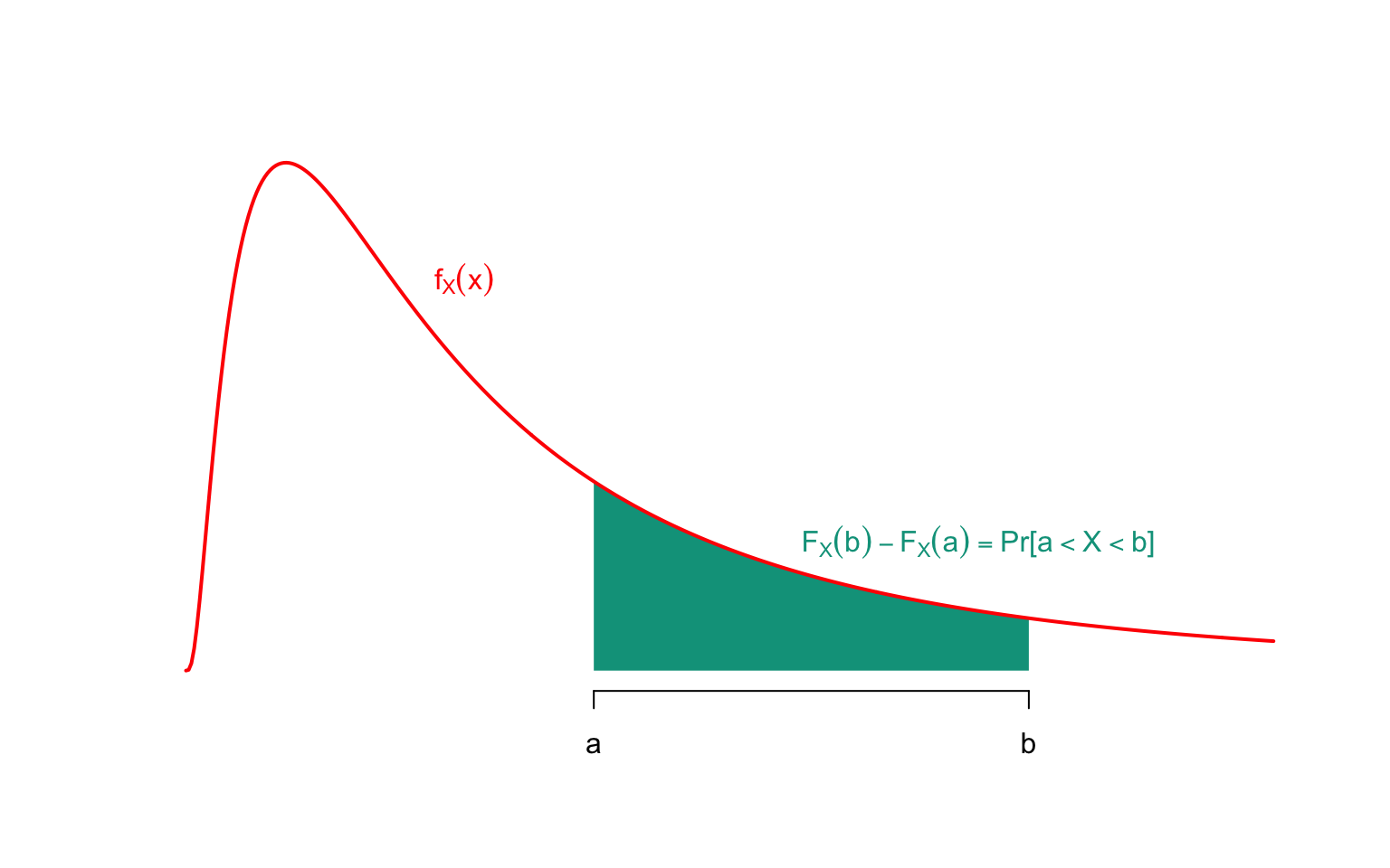
Figure 3.1: Graph of the density function \(f_X\) corresponding to a continuous variable \(X\)

We can easily deduce from the characteristics that all distribution functions must possess that the density \(f_X:{\mathbb{R}}\to{\mathbb{R}}^+\) must satisfy the condition \[ \int_{y\in{\mathbb{R}}}f_X(y)dy=1. \] Clearly, (3.9) guarantees that \[\begin{eqnarray*} f_X(x)&=&\frac{d}{dx}F_X(x)\\ &=&\lim_{\Delta x\to 0}\frac{F_X(x+\Delta x)-F_X(x)}{\Delta x} \\ &=&\lim_{\Delta x\to 0}\frac{Pr[x<X\leq x+\Delta x]}{\Delta x}, \end{eqnarray*}\]} so that the approximation \[ \Pr[x<X\leq x+\Delta x]\approx f_X(x)\Delta x \] is valid as long as \(\Delta x\) is sufficiently small. So, although \(f_X(x)\) is not a probability (and there’s no guarantee that \(f_X(x)\leq 1\)), the areas where \(f_X\) takes on very large values correspond to probable realizations of \(X\), while the areas where \(f_X\) takes on small values correspond to unlikely realizations of \(X\). If \(f_X=0\) on an interval \(I\), then the variable \(X\) cannot take any value in \(I\) (such areas correspond to a plateau for the graph of \(F_X\)).

Remark. It’s worth bearing in mind that continuous random variables are only approximations for easy calculations. Indeed, claims are expressed in euros, or even cents of a euro, but a value of 123.547324euro would be of little interest (as we could only pay out 123.55euro). In reality, then, all the random variables that make up the actuary’s daily routine are discrete. Those modeling the cost of claims take on so many possible values (in this case \(\frac{k}{100}\), \(k\in{\mathbb{N}}\)) that it’s more convenient to consider that all positive real values are possible. This brings us to the notion of continuous distribution and probability density described above.

In the remainder of this book, we shall use the following continuous distributions.

3.11.2 Continuous uniform distribution

The uniform (continuous) distribution appeared very early in statistics to model the result of pure chance, or phenomena about which no information was available. The first traces of uniform distribution date back to Bayes in 1763 and Laplace in 1872.

A random variable \(X\) is said to have a uniform distribution over the interval \([0,1]\) or to obey this distribution, which will henceforth be noted as \(X\sim\mathcal{U}ni(0,1)\), when \(X\) takes its values in this interval and admits the distribution function \[ F_X(x)=\left\{ \begin{array}{l} 0,\mbox{ if }x<0, \\ x,\mbox{ if }0\leq x<1, \\ 1,\mbox{ if }x\geq 1. \end{array} \right. \] The corresponding probability density is always equal to 1 on the unit interval, and zero elsewhere, i.e. \[ f_X(x)=\left\{ \begin{array}{l} 1,\mbox{ if }0\leq x\leq 1, \\ 0,\mbox{ otherwise} \end{array} \right. \]

The uniform distribution plays a special role in probability theory, because of the following result.

Proposition 3.4

1. If the distribution function \(F_X\) of \(X\) is continuous then \(F_X(X)\sim\mathcal{U}ni[0,1]\).
2. Let \(U\sim\mathcal{U}ni[0,1]\) and let \(X\) be any random variable. The random variable \(F_X^{-1}(U)\) has the same distribution as \(X\).

Proof.

1. Whatever \(t\) is in \((0,1)\), we have by Equation (3.6) \[\begin{eqnarray*} \Pr[F_X(X)\geq t]&=&\Pr[X\geq F_X^{-1}(t)]\\ &=&1-F_X\big(F_X^{-1}(t)\big)=1-t, \end{eqnarray*}\]} which shows that \(F_X(X)\) has a \(\mathcal{U}ni[0,1]\) distribution.
2. Whatever \(x\in {\mathbb{R}}\), we have by Equation (3.6) \[\begin{eqnarray*} \Pr[F_X^{-1}(U)\leq x] & = & \Pr[F_X(x)\geq U]=F_X(x), \end{eqnarray*}\] which completes the proof.

Remark. Point (2) of Proposition ?? is central to simulation. This approach, which we’ll describe in more detail later, involves recreating randomness by means of a computer, and enables us to solve problems for which an analytical solution is out of reach. The principle is simple to implement: if the computer is able to generate a sequence of numbers \(u_1,u_2,\ldots\) that is indistinguishable from a sequence of realizations of random variables \(\mathcal{U}ni[0,1]\), this sequence can easily be transformed into realizations of random variables with distribution function \(F_X\) by applying the transformation \(F_X^{-1}\) to them.

More generally, a uniform distribution over the interval \([a,b]\) is one whose probability density is constant over this interval and zero outside it. More precisely, a random variable is said to have a uniform distribution on the interval \([a,b]\), or to obey this distribution, which will henceforth be noted as \(X\sim\mathcal{U}ni[a,b]\), when the support of \(X\) is the interval in question and the density of \(X\) is given by \[ f_X(x)=\left\{ \begin{array}{l} \displaystyle\frac{1}{b-a},\text{ if }a\leq x\leq b,\\ 0,\text{ otherwise} \end{array} \right. \] Given a random variable \(U\sim\mathcal{U}ni[0,1]\), we can easily see that \[ \frac{X-a}{b-a}=_{\text{distribution}}U\Leftrightarrow X=_{\text{distribution}}a+(b-a)U. \]

3.11.3 Beta Distribution

Like the uniform distribution, the Beta distribution has an interval as its support, but does not assign to each interval contained in the support a probability mass proportional to its length. More precisely, a random variable \(X\) is said to have a Beta distribution with parameters \(\alpha>0\) and \(\beta>0\), which will henceforth be denoted \(X\sim\mathcal{B}et(\alpha,\beta)\), when \(X\) takes its values in the interval \([0,1]\) and admits the density \[ f_X(x)=\begin{cases} \displaystyle\frac{\Gamma(\alpha+\beta)}{\Gamma(\alpha)\Gamma(\beta)}x^{\alpha-1}(1-x)^{\beta-1},\text{ if }0\leq x\leq 1,\\ 0,\text{ otherwise} \end{cases} \]

From \(X\), we can easily construct a random variable \(Z\) that takes its values in the interval \([a,b]\) using the formula \(Z=a+(b-a)X\). It’s easy to check that the density of \(Z\) is given by \[ f_Z(x)= \begin{cases} \displaystyle\frac{\Gamma(\alpha+\beta)}{\Gamma(\alpha)\Gamma(\beta)(b-a)^{\alpha+\beta-1}}(z-a)^{\alpha-1}(b-z)^{\beta-1},\text{ if }a \leq z\leq b,\\ 0,\text{ otherwise} \end{cases} \]

Figure 3.2 shows the graph of probability densities associated with the \(\mathcal{B}et(\alpha,\beta)\) distributions, for different parameter values. It can be seen that the density can take on very different shapes depending on the parameter values.

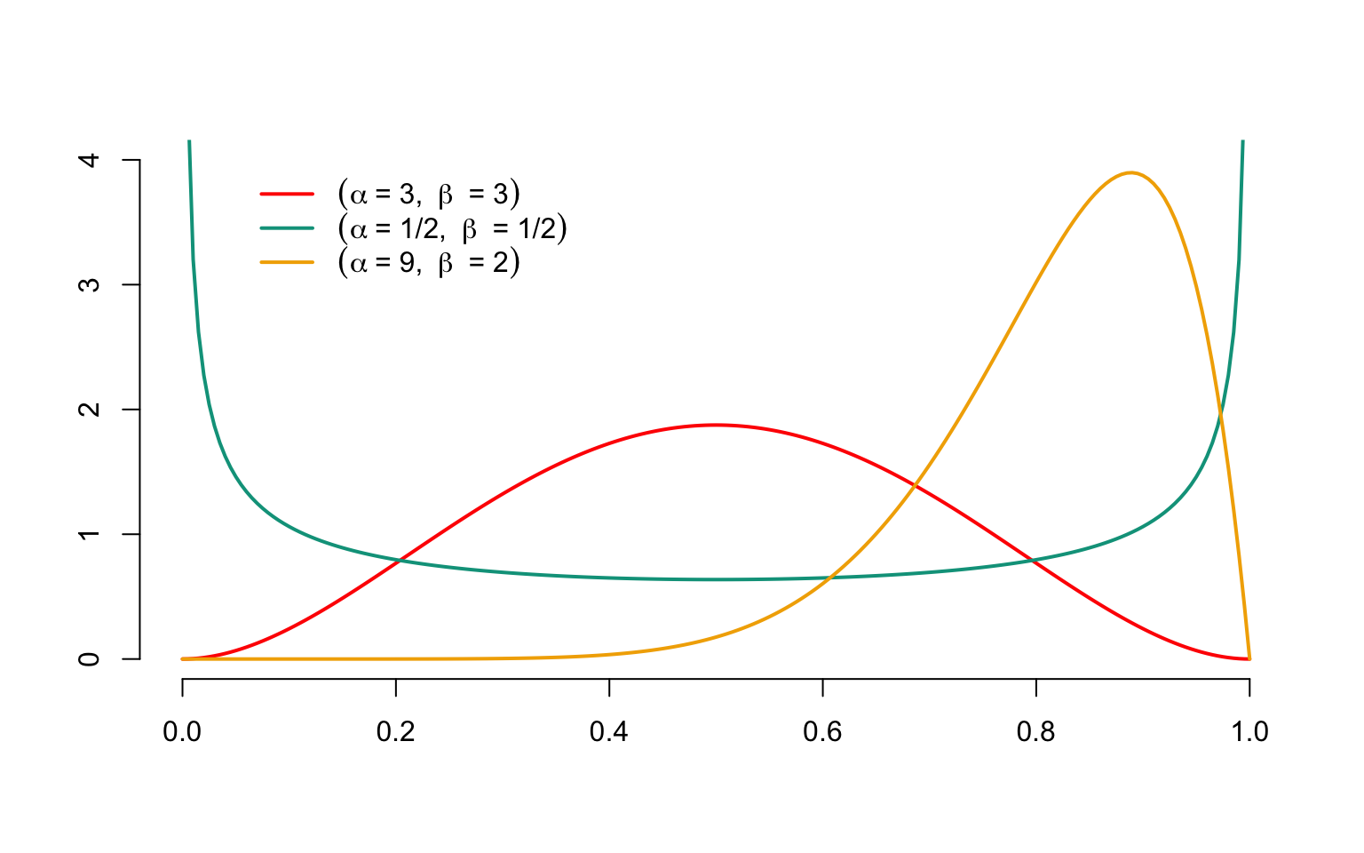
Figure 3.2: Densities of Beta ditributions with different values for \(\alpha\) and \(\beta\)

3.11.4 Normal (or Gaussian) distribution

The standard normal distribution is obtained from the following reasoning (linking the normal distribution to the theory of observation errors). The idea is to define a probability density expressing that the corresponding random variable takes small values around 0, symmetrically distributed with respect to the origin, and that large values are less likely the further away from the origin you are. We quickly come to postulate a density proportional to \(\exp(-x^2)\), which we then standardize so that the integral over \({\mathbb{R}}\) gives 1.

The normal distribution is undoubtedly one of the best-known (if not the best-known) in statistics. It first appeared as an approximation to the binomial distribution. In the early 19th century, its central role in theory was demonstrated by Laplace and Gauss. In astronomy, as in many other branches of the exact sciences, it plays a fundamental role in modeling measurement and observation errors.

A random variable \(X\) is said to have a Normal distribution with parameters \(\mu\in {\mathbb{R}}\) and \(\sigma>0\), or to obey this distribution, which is henceforth noted as \(X\sim\mathcal{N}or(\mu,\sigma^2)\), when \(X\) takes its values in \({\mathbb{R}}\) and admits the distribution function \[ x\mapsto \Pr[X\leq x]=\Phi\left(\frac{x-\mu}{\sigma}\right), \] where \(\Phi(\cdot)\) is the distribution function associated with the \(\mathcal{N}or(0,1)\) distribution given by \[ \Phi(x)=\frac{1}{\sqrt{2\pi}}\int_{y=-\infty}^x\exp(-y^2/2)dy, \hspace{2mm}x\in {\mathbb{R}}. \]

We can easily see that if \(X\sim\mathcal{N}or(\mu,\sigma^2)\) and if \(Z\sim\mathcal{N}or(0,1)\) then \(X=_{\text{distributio }}\mu+\sigma Z\). This explains the central role played by the \(\mathcal{N}or(0,1)\) distribution and its \(\Phi(\cdot)\) distribution function, known as the standard normal distribution, or centered reduced normal distribution.

We sometimes refer to a random variable obeying this distribution as \(\mathcal{N}or(\mu,\sigma^2)\). The probability density associated with \(\Phi\) is denoted \(\phi\) and is equal to \[ \frac{d}{dx}\Phi(x)=\phi(x)=\frac{1}{\sqrt{2\pi}}\exp(-\frac{x^2}{2}). \] Figure 3.3 shows the graph of probability densities associated with \(\mathcal{N}or(10,1)\), \(\mathcal{N}or(10,2)\) and \(\mathcal{N}or(10,3)\). The densities are clearly symmetrical with respect to $=$10 and the parameter \(\sigma^2\) controls the dispersion of possible values around \(\mu\): as \(\sigma^2\) increases, larger or smaller values relative to \(\mu\) become more likely. Generally speaking, the \(\phi\) density of the \(\mathcal{N}or(0,1)\) distribution is unimodal (maximum at \(\mu\)). It has two inflection points, in \(\mu\pm\sigma\).

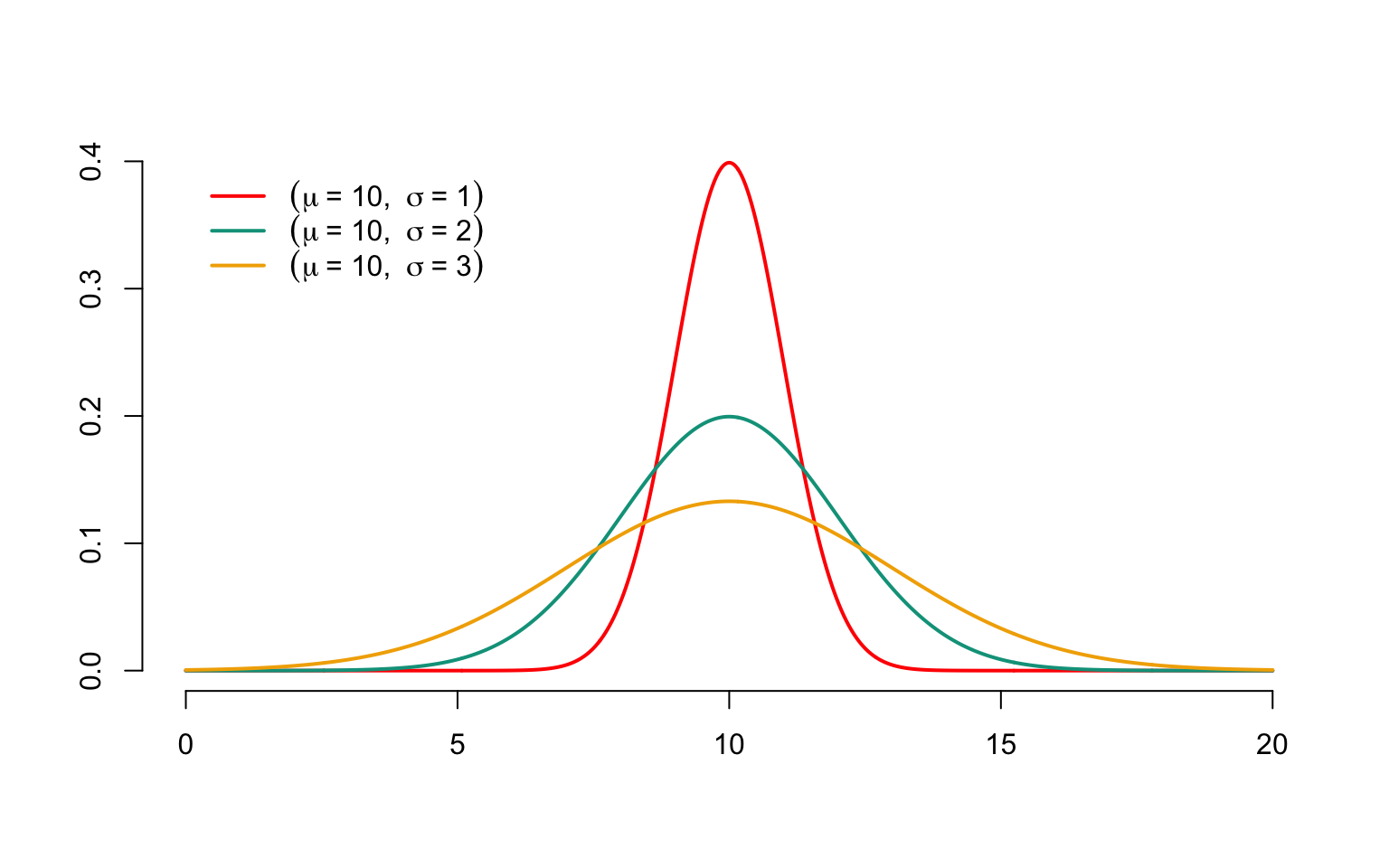
Figure 3.3: Densities of Gaussian distributions with parameters \(\mu=10\) and different values for \(\sigma^2\)

Remark. In recent decades, the limitations of classical Gaussian statistics have come to light, and the symmetry of the normal distribution has been severely criticized in many disciplines, including actuarial science. Nevertheless, most asymptotic results in statistics are based on the normal distribution, which is why this tool is so important.

3.11.5 Log-normal variable

As we have seen above, the normal distribution, because of its symmetry and the probability weight it gives to negative values, is not the ideal candidate for modeling claims costs. A simple solution to the problem would be to transform the variable to be modeled so that it better suits the actuary’s needs. Quite naturally, we can imagine using an exponential transformation, which leads to the log-normal distribution. More precisely, if \(Y\sim\mathcal{N}or(\mu,\sigma^2)\) and we define \(X=\exp Y\), for \(x>0\) we get, \[\begin{eqnarray*} \Pr[X\leq x] &=& \Pr[\exp Y\leq x]\\\\ & = & \Pr[Y\leq\ln x]\\\ & = & \Phi\left(\frac{\ln x-\mu}{\sigma}\right). \end{eqnarray*}\]t(). \end{eqnarray*}

This leads naturally to the following definition. A random variable \(X\) is said to have a Log-Normal distribution with parameters \(\mu\in{\mathbb{R}}\) and \(\sigma^2>0\), which will henceforth be denoted \(X\sim\mathcal{LN}or(\mu,\sigma^2)\), when \(X\) takes its values in \({\mathbb{R}}^+\) and admits the distribution function \[ F_X(x)=\left\{ \begin{array}{l} \Phi\left(\frac{\ln(x)-\mu} {\sigma}\right),\mbox{ if }x>0, \\ 0,\mbox{ otherwise}. \end{array} \right. \]

Lognormal distribution can be traced back to Francis Galton, who in 1879 introduced it as the limit distribution of a product of positive random variables. It was subsequently widely used in economics and finance.

The probability density of \(X\) is given by \[ f_X(x)=\left\{ \begin{array}{l} \frac{1}{x\sigma\sqrt{2\pi}}\exp\left(-\frac{1}{2}\left(\frac{\ln(x)-\mu} {\sigma}\right)^2\right),\mbox{ if }x>0, \\ 0,\mbox{ otherwise}. \end{array} \right. \] The quantile function is \[ F_X^{-1}(p)=\exp\big(\mu+\sigma\Phi^{-1}(p)\big). \] Figure 3.4 shows the probability density associated with the distribution \(\mathcal{LN}or(\mu,\sigma^2)\) for \(\mu=0\) and \(\sigma=0.5\), 1 and 1.5. The probability density is unimodal and the mode corresponds to \(\exp(\mu-\sigma^2)\).

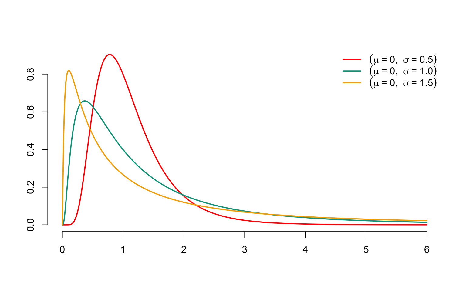
Figure 3.4: Densities of log-normal distributions with parameters \(\mu=0\) and different values for \(\sigma^2\).

3.11.6 (Negative) exponential distribution

A random variable \(X\) is said to have a (negative) exponential distribution (The term “negative exponential” is used to avoid any risk of confusion with the exponential family, a monument of modern statistics, which will be used in the chapter on generalized linear models) of parameter \(\theta>0\), or said to obey this distribution, which will henceforth be noted as \(X\sim\mathcal{E}xp(\theta)\), when \(X\) takes its values in \(\mathbb{R}^+\) and admits the probability density \[ f_X(x)= \begin{cases} \theta\exp(-\theta x),\mbox{ if }x>0, \\ 0,\mbox{ otherwise}. \end{cases} \]

The distribution function associated with the distribution \(\mathcal{E}xp(\theta)\) is given by \[ F_X(x)= \begin{cases} 1-\exp(-\theta x),\mbox{ if }x>0, \\ 0,\mbox{ otherwise}. \end{cases} \] The quantile function is \[ F_X^{-1}(p)=-\frac{1}{\theta}\ln(1-p). \]

By extension, we sometimes refer to a random variable obeying this distribution as \(\mathcal{E}xp(\theta)\). This is undoubtedly the most popular probability distribution in actuarial science. It has many interesting mathematical properties, which explains why actuaries are so fond of it. It should be borne in mind, however, that it reflects claims amounts that are relatively harmless for the company, with a thin distribution tail, since \({overline{F}_X(x)=\exp(-\theta x)\) exhibits exponential decay over \({\mathbb{R}}^+\).

Figure 3.5 shows the probability density associated with the \(\mathcal{E}xp(\theta)\) distribution for different values of \(\theta\). The probability density is unimodal and the mode is 0.

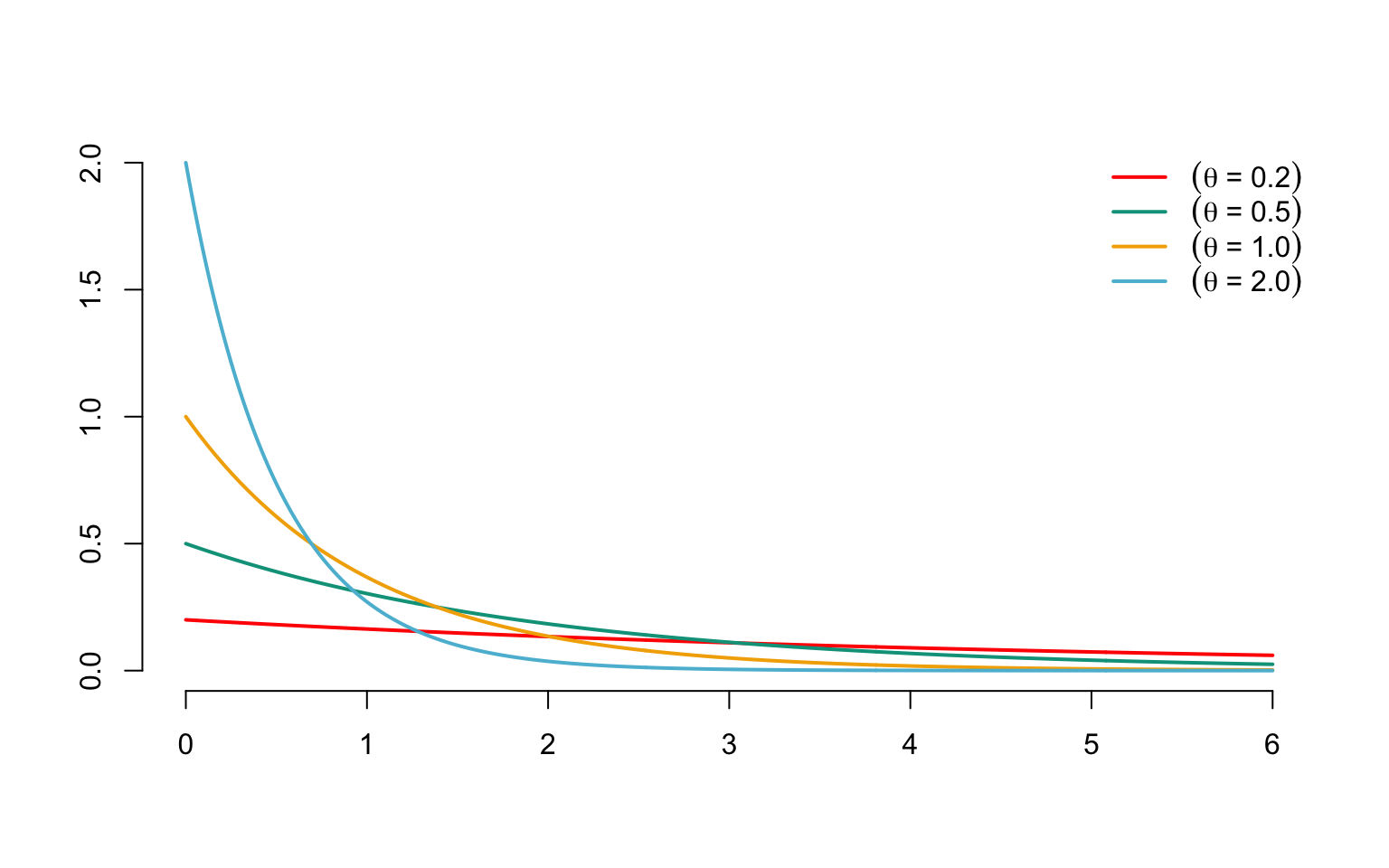
Figure 3.5: Densities of exponential distributions with different parameters \(\theta\)

3.11.7 Gamma distribution

The Gamma distribution was obtained by Laplace as early as 1836. Bienaymé demonstrated a special case (the chi-square or chi-squared distribution) in 1838 in relation to the multinomial distribution. A random variable \(X\) is said to have a Gamma distribution with parameters \(\alpha>0\) and \(\tau>0\), or to obey this distribution, which will henceforth be noted as \(X\sim\mathcal{G}am(\alpha,\tau)\), when \(X\) has the probability density \[ f_X(x)= \begin{cases} \displaystyle\frac{x^{\alpha-1}\tau^\alpha\exp(-x\tau)}{\Gamma(\alpha)},\mbox{ if }x\geq 0,\\ 0,\mbox{ otherwise} \end{cases} \] We sometimes refer to a random variable obeying this distribution as \(\mathcal{G}am(\alpha,\tau)\).

The tail function is written as \[ \overline{F}_X(x)=1-\Gamma(\alpha,\tau x), \] where \(\Gamma(\cdot,\cdot)\) is the incomplete Gamma function, defined by \[ \Gamma(t,\xi)=\frac{1}{\Gamma(t)}\int_{x=0}^\xi x^{t-1}\exp(-x)dx,\hspace{2mm}\xi,t\in{\mathbb{R}}^+. \]

Figure 3.6 shows the graph of \(f_X\) for different values of \(\alpha\) and \(\tau\). The mode is \((\alpha-1)/\tau\) when \(\alpha\geq 1\), and 0 otherwise. In addition, \[ \lim_{x\to 0}f_X(x)=+\infty,\text{ when }\alpha<1, \] and \[ \lim_{x\to 0}f_X(x)=0,\text{ when }\alpha=1. \]

We speak of a standard gamma distribution when \(\tau=1\); in this case, \[ f_X(x)=\frac{x^{\alpha-1}\exp(-x)}{\Gamma(\alpha)},\hspace{2mm}x\in{\mathbb{R}}^+. \] If \(X\) has a gamma distribution with parameters \(\alpha\) and \(\tau\), then \(\tau X\) has a standard gamma distribution with parameter \(\alpha\).

Remark. An interesting special case of the Gamma distribution is the chi-square (or chi-two) distribution with \(n\) degrees of freedom. This is the gamma distribution with parameters \(\alpha=n/2\) and \(\tau=1/2\).

Remark. When \(\alpha=1\), we find the negative exponential distribution, i.e. \(\mathcal{G}am(1,\tau)=\mathcal{E}xp(\tau)\).

Remark. When \(\alpha\) is a positive integer, this is sometimes referred to as an Erlang distribution. The distribution function is then given by \[ F_X(x)=1-\sum_{j=0}^{\alpha-1}\exp(-x\tau) \frac{(x\tau)^j}{j!},\hspace{2mm}x\geq 0. \]

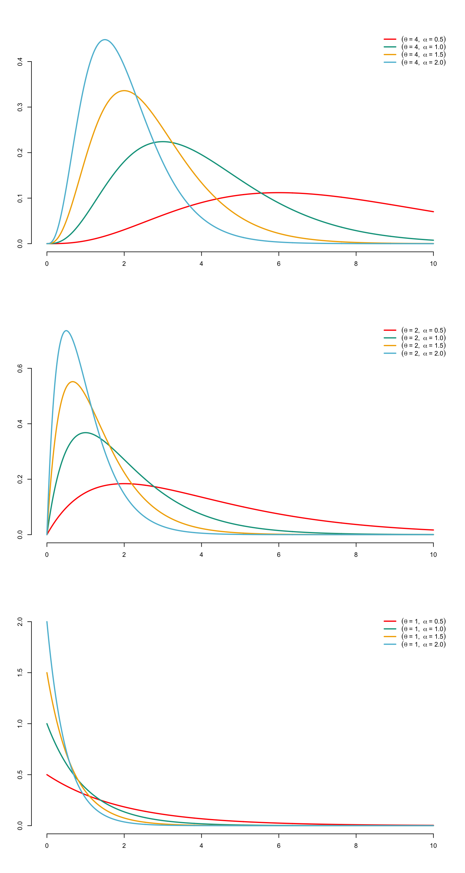
Figure 3.6: Densities of gamma distributions with parameters \(\tau=1/4\) (on top), 1/2 (in the middle) and 1 (belows) for differnt values for \(\alpha\)

3.11.8 Pareto distribution

This distribution takes its name from an Italian-born economics professor, Vilfredo Pareto, who introduced it in 1897 to model the distribution of income in a population. It can be obtained by transforming a random variable with a negative exponential distribution. Since the negative exponential distribution models claims that are not very dangerous for the company, we could consider that the amount of the claim \(X\) has the same distribution as \(\exp(Y)\), where \(Y\sim\mathcal{E}xp(\alpha)\). \[\begin{eqnarray*} \Pr[X\leq x] & = & \Pr[\exp(Y)\leq x]\\ & = & \Pr[Y\leq \ln x] \\ &=& \left\{ \begin{array}{l} 0,\mbox{ if }x\in]0,1],\\ 1-x^{-\alpha},\mbox{ if }x>1. \end{array} \right. \end{eqnarray*}\] This model represents a much less favorable situation for the insurer, since the tail function decreases polynomially (and no longer exponentially) towards 0. To obtain Pareto’s distribution, simply consider the distribution of the random variable \[ X=\theta\{\exp(Y)-1\},\text{ where }Y\sim\mathcal{E}xp(\alpha), \] whose survival function is \[\begin{eqnarray*} \Pr[X>x]&=&\Pr[Y>\ln(1+(x/\theta))]\\ &=&\left(1+\frac{x}{\theta}\right)^{-\alpha}\\ &=&\left(\frac{\theta}{x+\theta}\right)^\alpha. \end{eqnarray*}\] Thus, a random variable \(X\) is said to have a Pareto distribution with parameters \(\alpha>0\) and \(\theta>0\), which will henceforth be denoted \(X\sim\mathcal{P}ar(\alpha,\theta)\), when \(X\) admits the distribution function \[ F_X(x)=\left\{ \begin{array}{l} 1-\left(\displaystyle\frac{\theta}{x+\theta}\right)^\alpha, \mbox{ if }x\geq 0, \\ 0,\mbox{ otherwise} \end{array} \right. \] Pareto’s distribution defined in this way is sometimes called Lomax’s distribution (or Type II Pareto’s distribution). From now on, we’ll sometimes refer to a random variable obeying this distribution as \(\mathcal{P}ar(\alpha,\theta)\). The quantile function is \[ F_X^{-1}(p)=\theta\big((1-p)^{-1/\alpha}-1\big). \]

Pareto’s distribution is considered to be one of the most dangerous for the insurer (since the probability of the claim amount exceeding \(x\) decreases polynomially with the amount \(x\), whereas the decrease is exponential with the other models introduced above). This explains its frequent use in reinsurance. The probability density associated with the Pareto distribution is given by \[ f_X(x)=\left\{ \begin{array}{l} \frac{\alpha\theta^\alpha}{(x+\theta)^{\alpha+1}}, \mbox{ if }x\geq 0, \\ 0,\mbox{ otherwise,} \end{array} \right. \] where \(\alpha>0\), \(\theta>0\); \(f_X\) is clearly unimodal (the unique mode is in 0). See Figure 3.7 for a graph of \(f_{alpha,\theta}\) and different parameter values.

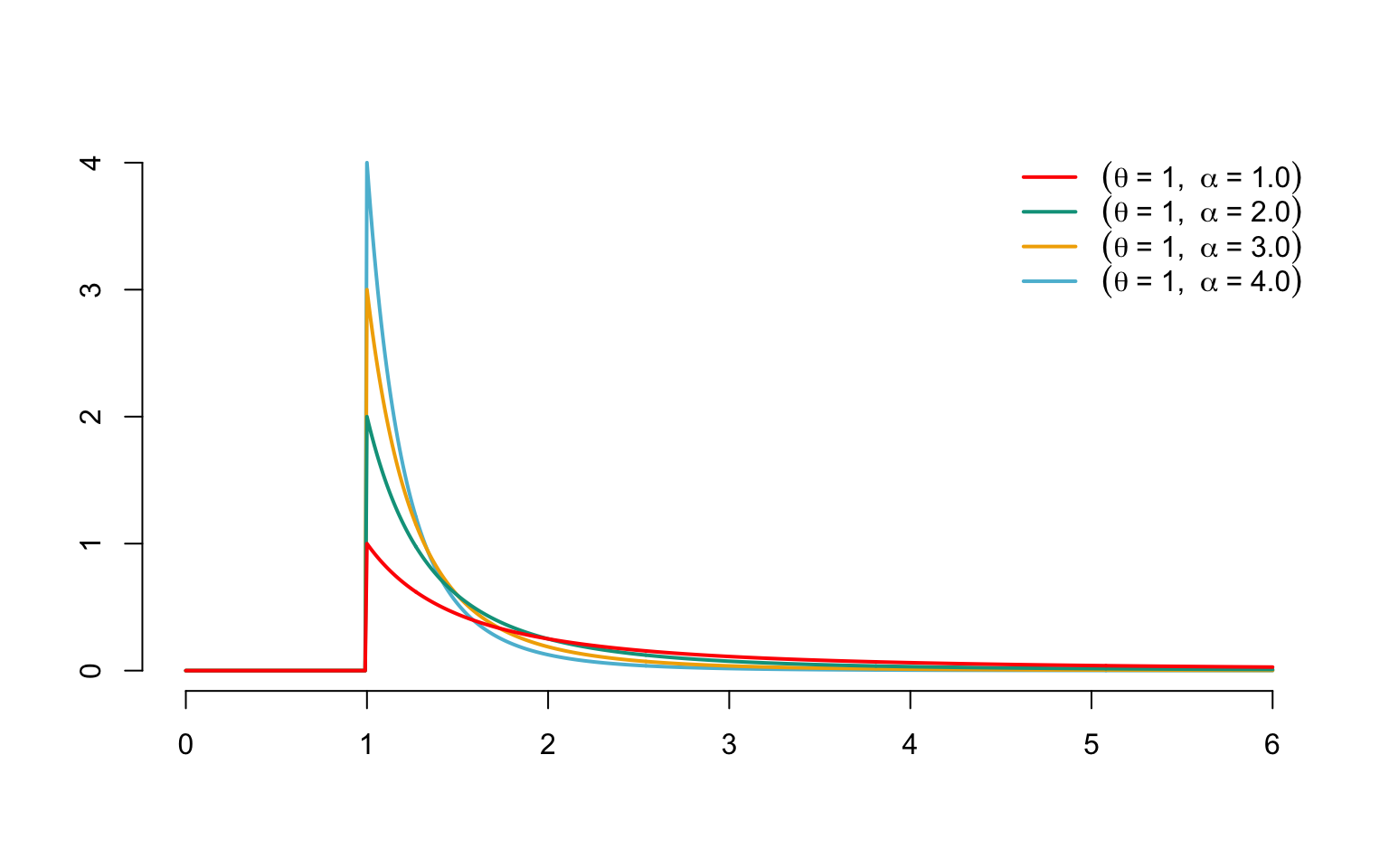
Figure 3.7: Densities of Pareto distributions with \(\theta=1\) and different values for \(\alpha\)

Remark. Later on, we’ll come across a slightly different version of Pareto’s distribution, known as the generalized Pareto distribution, which appears naturally in the study of the behavior of the maximum of \(n\) random variables, when \(n\to +\infty\).

3.12 Random vector

3.12.1 Definition

A random vector \(\boldsymbol{X}\) is the result of the union of \(n\) random variables \(X_1,X_2,\ldots,X_n\) defined on the same probability space \((\mathcal{E},\mathcal{A},\Pr)\). In the following, we will always consider \(\boldsymbol{X}\) as a column vector: \[ \boldsymbol{X}=\left(\begin{array}{c} X_1\\ X_2\\ \vdots\\ X_n \end{array} \right) =(X_1,X_2,\ldots,X_n)^\top, \] where the superscript “\(\top\)” indicates the transposition.

3.12.2 Distribution function

3.12.2.1 General definition

As with random variables, the stochastic behavior of a vector \(\boldsymbol{X}\) is fully described by its joint distribution function \(F_{\boldsymbol{X}}\), defined as follows.

Definition 3.8 The distribution function \(F_{\boldsymbol{X}}\) associated with the random vector \(\boldsymbol{X}\) is defined as follows: \[\begin{eqnarray*} F_{\boldsymbol{X}}(\boldsymbol{x})&=& \Pr\big[\{e\in\mathcal{E}|X_1(e)\leq x_1,X_2(e)\leq x_2,\ldots,X_n(e)\leq x_n\}\big]\\ &=&\Pr[X_1\leq x_1,X_2\leq x_2,\ldots,X_n\leq x_n],\boldsymbol{x}\in{\mathbb{R}}^n. \end{eqnarray*}\]

In the light of this definition, \(F_{\boldsymbol{X}}(\boldsymbol{x})\) is therefore the probability that, simultaneously, each of the \(X_i\) components of the \(\boldsymbol{X}\) vector is lower than the corresponding \(x_i\) level. It is therefore the premium to be paid to receive a 1payment if the variables \(X_1,\ldots,X_n\) are simultaneously below the thresholds \(x_1,\ldots,x_n\).

From now on, we’ll often use vector notation. For example, the event \(\{\boldsymbol{X}\leq \boldsymbol{x}\}\) is equivalent to the event \(\{X_1\leq x_1,\ldots,X_n\leq x_n\}\).

3.12.2.2 In dimension 2

We saw in Property 3.1 what conditions a univariate distribution function must satisfy. This result can be generalized to the \(2\) dimension as follows.

Proposition 3.5 \(F_{\boldsymbol{X}}\) is the distribution function of a \(\boldsymbol{X}\) pair if, and only if, \(F_{\boldsymbol{X}}\)

• is non-decreasing
• is continuous on the right
• satisfies \[\begin{eqnarray*} \lim_{t\to -\infty}F_{\boldsymbol{X}}(x_1,t)&=&0,\text{ whatever }x_1\in{\mathbb{R}},\\ \lim_{t\to -\infty}F_{\boldsymbol{X}}(t,x_2)&=&0,\text{ whatever }x_2\in{\mathbb{R}},\\ \lim_{x_1,x_2\to +\infty}F_{\boldsymbol{X}}(x_1,x_2)&=&1, \end{eqnarray*}\] as well as \[\begin{eqnarray} &&F_{\boldsymbol{X}}(x_1+\delta,x_2+\epsilon)-F_{\boldsymbol{X}}(x_1+\delta,x_2)\nonumber\\ &&-F_{\boldsymbol{X}}(x_1,x_2+\epsilon)+F_{\boldsymbol{X}}(x_1,x_2)\geq 0 \tag{3.10} \end{eqnarray}\] whatever \(\boldsymbol{x}\in{\mathbb{R}}^2\) and \(\epsilon\), \(\delta>0\).

Remark. The condition (3.10) is still equivalent, in the case where \(F_{\boldsymbol{X}}\) is twice derivable, to \[ \frac{\partial ^{2}}{\partial x_1\partial x_2}F_{\boldsymbol{X}}(\boldsymbol{x})\geq 0. \]

In general, (3.10) guarantees that the probability of \(\boldsymbol{X}\) taking a value in the rectangle of vertices \((x_1,x_2)\), \((x_1+\delta,x_2)\), \((x_1,x_2+\epsilon)\) and \((x_1+\delta,x_2+\epsilon)\) is always positive. In the rest of this book, we’ll refer to the same type of constraint as the (3.10) inequality as supermodularity.

3.12.2.3 Any dimension

Let’s now look at the properties required of any distribution function in any dimension. This is an immediate generalization of Property 3.5, except for the (3.10) condition, which becomes a little more complicated.

Proposition 3.6 \(F_{\boldsymbol{X}}\) is the distribution function of a \(n\)-dimensional random vector \(F_{\boldsymbol{X}}\) if, and only if, \(F_{\boldsymbol{X}}\)

• is non-decreasing;
• is continuous on the right;
• satisfies \[\begin{eqnarray*} \lim_{x_j\to -\infty}F_{\boldsymbol{X}}(x_1,x_2,\ldots,x_n)&=&0, \mbox{ for }j=1,2,\ldots,n,\\ \lim_{x_1,x_2,\ldots,x_n\to +\infty}F_{\boldsymbol{X}}(x_1,x_2,\ldots,x_n)&=&1, \end{eqnarray*}\] and, whatever \((\alpha_1,\alpha_2,\ldots,\alpha_n),(\beta_1,\beta_2,\ldots,\beta_n)\in {\mathbb{R}}^n\), with \(\alpha_i\leq \beta_i\) for \(i=1,2,\ldots,n\), defining: \[\begin{eqnarray*} \Delta_{\alpha_i,\beta_i}F_{\boldsymbol{X}}(\boldsymbol{x}) &=&F_{\boldsymbol{X}}(x_1,\ldots,x_{i-1},\beta_i,x_{i+1},\ldots, x_n)\\ & &-F_{\boldsymbol{X}}(x_1,\ldots,x_{i-1},\alpha_i,x_{i+1},\ldots, x_n), \end{eqnarray*}\] \[ \Delta_{\alpha_1,\beta_1}\Delta_{\alpha_2,\beta_2}\ldots\Delta_{\alpha_n,\beta_n}F_{\boldsymbol{X}}(\boldsymbol{x})\geq 0. \]

Remark. As in dimension 2, the inequality in Property 3.6 guarantees that: \[ \Pr[\boldsymbol{\alpha}\leq\boldsymbol{X}\leq\boldsymbol{\beta}]\geq 0\mbox{ for all } \boldsymbol{\alpha}\leq\boldsymbol{\beta}\in {\mathbb{R}}^n. \] When \(F_{\boldsymbol{X}}\) is sufficiently regular, the inequality in Property 3.6 is still equivalent to \[ \frac{\partial^n}{\partial x_1\partial x_2\ldots\partial x_n} F_{\boldsymbol{X}}(\boldsymbol{x})=f_{\boldsymbol{X}}(\boldsymbol{x})\geq 0\mbox{ on } {\mathbb{R}}^n, \] where \(f_{\boldsymbol{X}}\) is the joint probability density of the vector \(\boldsymbol{X}\). We then have \[ F_{\boldsymbol{X}}(\boldsymbol{x})=\int_{-\infty}^{x_1}\ldots \int_{-\infty}^{x_n}f_{\boldsymbol{X}}(\boldsymbol{y})dy_1\ldots dy_n. \]

3.12.2.4 Marginal distribution functions

The behavior of each \(X_j\) component is described by the corresponding \(F_{X_j}\) distribution function. The functions \(F_{X_1}\), \(F_{X_2}\), \(\ldots\), \(F_{X_n}\) are called marginal distribution functions. Clearly, \[ \lim_{x_i\to +\infty\text{ for all }i\neq j}F_{\boldsymbol{X}}(\boldsymbol{x})=F_{X_j}(x_j). \]

3.12.3 Support of vector \(\boldsymbol{X}\)

The support \(\mathcal{S}_{\boldsymbol{X}}\) of the random vector \(\boldsymbol{X}\) is defined as the subset of \({\mathbb{R}}^n\) containing the points \(\boldsymbol{x}\) where \(F_{\boldsymbol{X}}\) is strictly increasing. \(\mathcal{S}_{\boldsymbol{X}}\) is included in the hyper-rectangle \[ \Big[F_{X_1}^{-1\bullet}(0),F_{X_1}^{-1}(1)\Big]\times \Big[F_{X_2}^{-1\bullet}(0),F_{X_2}^{-1}(1)\Big]\times \ldots \Big[F_{X_n}^{-1\bullet}(0),F_{X_n}^{-1}(1)\Big] \] where \(F_{X_i}\), \(i=1,2,\ldots,n\), are the marginals of \(F_{\boldsymbol{X}}\).

3.12.4 Independence

Often, the actuary will be confronted with several random variables \(X_1,X_2,X_3,\ldots\) (representing, for example, the insurer’s expense for different policies in the portfolio). It is then important to know whether the value taken by one of these variables could influence those taken by the others.

Example 3.9 If we consider the insurance of buildings against earthquakes, and if \(X_1\) and \(X_2\) represent two risks of the same characteristics located in the same geographical area, we would be tempted to say that if \(X_1\) takes on a large value (meaning that the first building has suffered significant damage from the earthquake), \(X_2\) should also take on a high value. Conversely, a small value of \(X_1\) could mean that \(X_2\) is also likely to be quite small (since a small value of \(X_1\) makes a low-magnitude earthquake more likely). In such a situation, the risks \(X_1\) and \(X_2\) are said to be positively dependent.

Another classic situation is when the value of \(X_1\) has no influence on that of \(X_2\).

Example 3.10 Consider, for example, two fire hazards located in different regions. It’s hard to see how the consequences of a fire affecting one of the buildings could provide information about a hypothetical loss affecting the other.

Intuitively, random variables \(X_1,X_2,\ldots,X_n\) are mutually independent if the value of any one of them does not influence the others.

Definition 3.9 Formally, random variables \(X_1,\ldots,X_n\) are independent when \[\begin{eqnarray} &&\Pr[X_i\leq x_i\text{ for }i\in\mathcal{I}|X_j\leq x_j\text{ for }j\in\mathcal{J}]\nonumber\} &=&\Pr[X_i\leq x_i\text{ for }i\in\mathcal{I}] \tag{3.11} \end{eqnarray}\] whatever the reals \(x_i\) and \(x_j\), and the subsets \(\mathcal{I}\) and \(\mathcal{J}\) disjoint from \(\{1,\ldots,n\}\).

This reflects the idea that knowing that \(X_j\), \(j\in\mathcal{J}\), are small (i.e. below the \(x_j\) thresholds) tells us nothing about the probability that \(X_i\), \(i\in\mathcal{I}\), are also small (i.e. below the \(x_i\) thresholds). More generally, (3.11) guarantees that the occurrence of any event involving \(X_j\), \(j\in\mathcal{J}\), has no influence on the probability of any event involving \(X_i\), \(i\in\mathcal{I}\), occurring.

The only way equality (3.11) can be satisfied is if the joint distribution function of the vector \(\boldsymbol{X}\) factorizes into the product of its marginals.

Proposition 3.7 The random variables \(X_1,X_2,\ldots,X_n\) are independent if, and only if, the factorization \[ F_{\boldsymbol{X}}(\boldsymbol{x})=\prod_{i=1}^nF_{X_i}(x_i)\mbox{ holds for all }\boldsymbol{x}\in {\mathbb{R}}^n. \]

Independence can also be verified using probability densities.

Proposition 3.8

1. If \(X_i\) are continuous, the random variables \(X_1,\ldots,X_n\) are independent if, and only if, their joint probability density factorizes, i.e. \[ f_{\boldsymbol{X}}(\boldsymbol{x}) %=\frac{\partial^n}{\partial x_1\ldots\partial x_n}F_{\Xvec}(\xvec) =\prod_{i=1}^nf_{X_i}(x_i). \]
2. If \(X_i\) are count variables, so are the joint probabilities, i.e. \[ \Pr[X_1=k_1,\ldots,X_n=k_n]=\prod_{i=1}^n\Pr[X_i=k_i]. \]

3.12.5 Gaussian vector

A random variable with a \(\mathcal{N}or(\mu,\sigma^2)\) distribution has a density that can be expressed as \[ f_X(x) = \frac{1}{\sigma\sqrt{2\pi}} \exp \left\{ -\frac{1}{2} Q_1(x;\mu,\sigma^2) \right\}, \quad x \in {\mathbb{R}}, \] with \[ Q_1(x;\mu,\sigma^2) = \frac{1}{\sigma^2} (x-\mu)^2 = (x-\mu)(\sigma^2)^{-1}(x-\mu) \] where \(\mu \in {\mathbb{R}}\) and \(\sigma^2 > 0\). Let’s extend this definition to the bivariate case. Given a pair of real numbers \[ {\boldsymbol{\mu}} = \left( \begin{array}{c} \mu_1\\\mu_2 \end{array} \right) \] and a matrix \[ {\boldsymbol{\Sigma}} = \left( \begin{array}{cc} \sigma_1^2 & \sigma_{12} \\ \sigma_{12} & \sigma_2^2 \end{array} \right) \] such that \(\sigma_i^2 > 0\), \(i=1,2\), \(|\sigma_{12}|<\sigma_1\sigma_2\). From now on, we’ll denote \(|\boldsymbol{\Sigma}|\) the determinant of the \(\boldsymbol{\Sigma}\) matrix. A random pair \({\boldsymbol{X}} = (X_1,X_2)\) is said to have a normal distribution, which will henceforth be denoted \({\boldsymbol{X}}sim\mathcal{N}or(\boldsymbol{\mu},\boldsymbol{\Sigma})\), if it admits a density of the form \[ f_{\boldsymbol{X}}({\boldsymbol{x}}) = \frac{1}{2\pi|{\boldsymbol{\Sigma}}|^{1/2}}\exp\left[ -\frac{1}{2} Q_2({\boldsymbol{x}};{\boldsymbol{\mu}},{\boldsymbol{\Sigma}})\right],~{\boldsymbol{x}}\in {\mathbb{R}}^2 \] where \[ Q_2({\boldsymbol{x}};{\boldsymbol{\mu}},{\boldsymbol{\Sigma}}) = ({\boldsymbol{x}}-{\boldsymbol{\mu}})^{t}{\boldsymbol{\Sigma}}^{-1}({\boldsymbol{x}}-{\boldsymbol{\mu}}) \] Figure 3.8 shows different graphs of the bivariate probability density associated with the normal distribution for \(\boldsymbol{\mu}=(0,0)^\top\), \(\sigma_1^2=\sigma_2^2=1\) and different values of \(\sigma_{12}\).

Remark. In some cases, the \(\boldsymbol{\Sigma}\) matrix is not invertible, and we have to adapt the definition of the \(\mathcal{N}or(\boldsymbol{\mu},\boldsymbol{\Sigma})\) distribution (since inversion in \(Q_2\) is no longer allowed). More precisely, \({\boldsymbol{X}}\) is said to have a singular normal distribution (singular because the \(\boldsymbol{\Sigma}\) matrix is singular, i.e. non-invertible) if there are real numbers \(\sigma_1\), \(\sigma_2\), \(\mu_1\) and \(\mu_2\) such that \({\boldsymbol{X}}=_{\text{distribution}}(\sigma_1 Z + \mu_1, \sigma_2 Z + \mu_2)\), where \(Z\sim\mathcal{N}or(0,1)\).

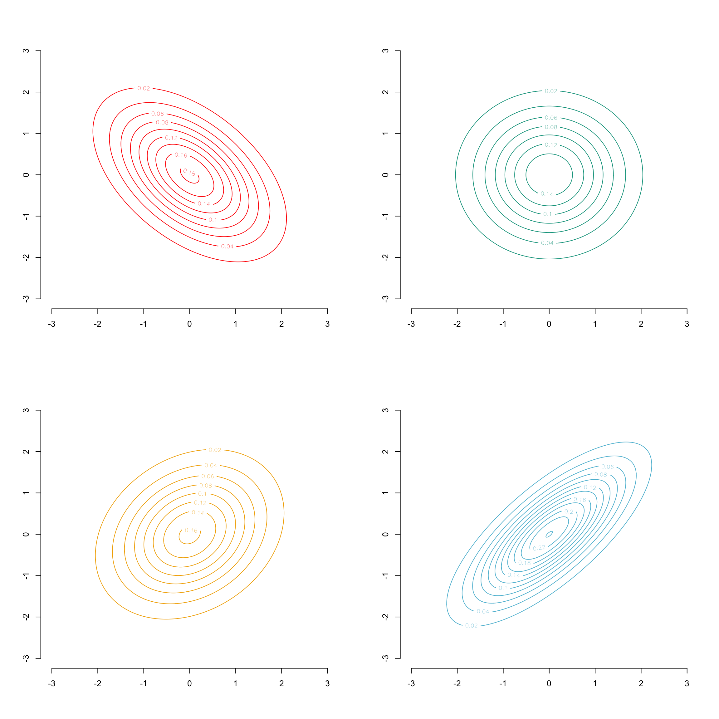
Figure 3.8: Density of the bivariate Gaussian distribution with parameters \(\boldsymbol{\mu}=(0,0)^\top\), \(\sigma_1^2=\sigma_2^2=1\) and different values for \(\sigma_{12}\)

The definitions given above are easily extended to any dimension (by substituting a \(n\)-dimensional vector for the \(\boldsymbol{\mu}\) pair and a symmetrical positive-definite \(n\times n\)-square matrix for the \(2\times 2\) \(\boldsymbol{\Sigma}\) matrix, and dividing by \((2\pi)^{n/2}\)).

The following property indicates that the parameter \(\sigma_{12}\) is the one controlling the possible dependency between \(X_1\) and \(X_2\).

Proposition 3.9 When \(\sigma_{12}=0\), the components of \(\boldsymbol{X}\sim\mathcal{N}or(\boldsymbol{\mu},\boldsymbol{\Sigma})\) are independent.

Proof. When \(\sigma_{12}=0\), \(Q_2\) equals \[\begin{eqnarray*} Q_2({\boldsymbol{x}};{\boldsymbol{\mu}},{\boldsymbol{\Sigma}}) &=& ({\boldsymbol{x}}-{\boldsymbol{\mu}})^{t}\frac{1}{\sigma_1^2\sigma_2^2} \left(\begin{array}{cc}\sigma_2^2&0\\0&\sigma_1^2\end{array}\right)({\boldsymbol{x}}-{\boldsymbol{\mu}})\\ &=&\frac{1}{\sigma_1^2}(x_1-\mu_1)^2+\frac{1}{\sigma_2^2}(x_2-\mu_2)^2. \end{eqnarray*}\]} Therefore, the joint density \[\begin{eqnarray*} f_{\boldsymbol{X}}(\boldsymbol{x})&=&\frac{1}{\sigma_1\sqrt{2\pi}} \exp \left\{ -\frac{1}{2} Q_1(x_1;\mu_1,\sigma_1^2) \right\} \\ &&\times\frac{1}{\sigma_2\sqrt{2\pi}} \exp \left\{ -\frac{1}{2} Q_1(x_2;\mu_2,\sigma_2^2) \right\} \end{eqnarray*}\] factorizes into the product of the densities associated with \(X_1\) and \(X_2\).

Remark. The generally accepted definition of the multivariate Gaussian distribution is as follows. A vector \(\boldsymbol{X}=(X_1,\ldots,X_n)\) is said to be Gaussian when any linear combination \(\sum_{j=1}^n\alpha_jX_j\) of its components is of univariate normal distribution (with the convention of \(\mathcal{N}or(\mu,0)\) designating a unit probability mass placed in \(\mu\)). In particular, each component \(X_1,\ldots,X_n\) has a normal distribution.

Remark. Note that for a vector to be Gaussian, it is not sufficient for its marginals to be normal. Indeed, if we consider the pair \((X_1,X_2)\) such that \(X_1\sim\mathcal{N}or(0,1)\) and \[ X_2=\begin{cases} X_1,\text{ if }|X_1|\leq 1\\ -X_1,\text{ otherwise}, \end{cases} \] we have \(X_2\sim\mathcal{N}or(0,1)\), but \((X_1,X_2)\) is not a Gaussian vector since the line \(x_1=-x_2\) is assigned a probability mass \[ 0<\Pr[X_1+X_2=0]<1, \] which means that \(X_1+X_2\) cannot have a normal distribution.

The \(\mathcal{N}or(\boldsymbol{\mu},\boldsymbol{\Sigma})\) distribution can be obtained from the standard (or centered-reduced) normal distribution \(\mathcal{N}or(\boldsymbol{0},\text{Id})\) (i.e. the distribution of a vector whose components are independent and have the same \(\mathcal{N}or(0,1)\) distribution) using the following result.

Proposition 3.10 Let \(\boldsymbol{X}\sim\mathcal{N}or(\boldsymbol{\mu},\boldsymbol{\Sigma})\) and \(\boldsymbol{Z}\sim\mathcal{N}or(\boldsymbol{0},\text{Id})\). By defining the matrix \(\boldsymbol{T}\) such that \(\boldsymbol{T}^\top\boldsymbol{T}=\boldsymbol{\Sigma}\), we have \(\boldsymbol{X}=_{\text{distribution}}\boldsymbol{\mu}+\boldsymbol{T}^\top\boldsymbol{Z}\).

3.12.6 Elliptical vectors

3.12.7 Definition

Elliptical distributions were introduced by Kelker in 1970. Spherical distributions are generalizations of the distribution $or( ,) $ and elliptical distributions are generalizations of the distribution $or( ,) $.

Definition 3.10 A random vector \(\boldsymbol{X}\) of \({\mathbb{R}}^{n}\) is said to have an elliptical distribution of generator \(g\) and parameters \(\boldsymbol{\mu}\) and \(\boldsymbol{\Sigma}\), which will henceforth be denoted \(\boldsymbol{X}\sim\mathcal{E}ll(g,\boldsymbol{\mu},\boldsymbol{\Sigma})\) when it admits the density \[\begin{equation} f_{\boldsymbol{X}}\left( \boldsymbol{x}\right) =\frac{c_{n}}{{\left| \boldsymbol{\Sigma}\right| }^{1/2}} g\left( \frac{1}{2}\left( \boldsymbol{x}-\boldsymbol{\mu}\right) ^\top\boldsymbol{\Sigma}^{-1} \left( \boldsymbol{x}-\boldsymbol{\mu}\right) \right) , \tag{3.12} \end{equation}\] where the normalization constant \(c_{n}\) is given by%. \[\begin{equation*} c_{n}=\frac{\Gamma \left( n/2\right) }{\left( 2\pi \right) ^{n/2}} \int_{0}^{\infty }t^{n/2-1}g\left( t\right)dt . \end{equation*}\]

Remark. If we take \(g\) to be the exponential function, we see that the multivariate normal distribution \(\mathcal{N}or(\boldsymbol{\mu},\boldsymbol{\Sigma})\) is found.

3.12.7.1 Marginal behavior

The marginals of elliptical distributions are themselves elliptical, i.e.
\[ \boldsymbol{X}\sim\mathcal{E}ll(g,\boldsymbol{\mu},\boldsymbol{\Sigma})\Rightarrow X_k\sim\mathcal{E}ll(g,\mu_k,\sigma_k^2)\text{ for }k=1,\ldots,n. \] Moreover, whatever the matrix \(\boldsymbol{B}\) and the vector \(\boldsymbol{b}\), \[ \boldsymbol{X}\sim\mathcal{E}ll(g,\boldsymbol{\mu},\boldsymbol{\Sigma})\Rightarrow \boldsymbol{X}\sim\mathcal{E}ll(g,\boldsymbol{b}+\boldsymbol{B}\boldsymbol{\mu}, \boldsymbol{B}\boldsymbol{\Sigma}\boldsymbol{B}^\top). \]

3.12.7.2 Multivariate Student \(t\)’s distribution

The multivariate Student’s distribution is obtained with the generator in dimension \(n\), \[\begin{equation*} g\left( t\right) =\left( 1+\frac{t}{k_{p}}\right) ^{-p}, \end{equation*}\] where parameter \(p\) is greater than \(n/2\), and \(k_{p}\) is a normalization constant.

The density of \(\boldsymbol{x}\) is then given by \[\begin{equation*} f_{\boldsymbol{X}}\left( \boldsymbol{x}\right) =\frac{c_{n}}{{\left| \boldsymbol{\Sigma} \right| }^{1/2}}\left[ 1+\frac{\left( \boldsymbol{x}-\boldsymbol{\mu}\right) ^\top\boldsymbol{\Sigma} \left( \boldsymbol{x}-\boldsymbol{\mu}\right) }{\Gamma \left( p-n/2\right) }\right] ^{-p}\text{ for }\boldsymbol{x}\in {\mathbb{R}}^{n}. \end{equation*}\]

The multivariate Student’s distribution can also be obtained using the the following construction, in terms of random variables.

Proposition 3.11 Let $or(,) $ and \(S\) have mutually independent chi-square distributions with \(m\) degrees of freedom. The vector \(\boldsymbol{Y}=\sqrt{m}\boldsymbol{Z}/S\) obeys multivariate Student’s distribution, with \(m\) degrees of freedom. This can be generalized by considering \(\boldsymbol{Y}^{\ast }=\boldsymbol{\mu}+\boldsymbol{T}^\top\boldsymbol{Y}\), where \(\boldsymbol{T}^\top\boldsymbol{T}=\boldsymbol{\Sigma}\).

3.12.7.3 Multivariate Cauchy’s distribution

The multivariate Cauchy distribution has the density \[\begin{equation*} f_{vec}\left( \boldsymbol{x}\right) =\frac{\Gamma \left( \left( n+1\right) /2\right) }{\pi ^{\left( n+1\right) /2}{\left| \boldsymbol{\Sigma} \right| }^{1/2}}\Big( 1+\left( \boldsymbol{x}-\boldsymbol{\mu}\right) ^\top\boldsymbol{\Sigma}\left( \boldsymbol{x}-\boldsymbol{\mu}\right) \Big) ^{-\left( n+1\right) /2}\text{ for }\boldsymbol{x}\in {\mathbb{R}}^{n}. \end{equation*}\]

3.12.7.4 Multivariate logistic distribution

The multivariate logistic distribution admits the generator \[ g\left( t\right) =\frac{\exp(-t)}{\big(1+\exp(-t)\big) ^{2}}. \] The density is then \[ f_{\boldsymbol{x}}\left(\boldsymbol{x}\right) =\frac{c_{n}}{{\left| \boldsymbol{\Sigma}\right| }^{1/2}}\frac{\exp\left( -\frac{1}{2}\left(\boldsymbol{x}-\boldsymbol{\mu}\right)^\top\Sigma^{-1}\left(\boldsymbol{x}-\boldsymbol{\mu}\right)\right)}{\big( 1+\exp\left(-\frac{1}{2}\left( \boldsymbol{x}-\boldsymbol{\mu}\right)^\top\boldsymbol{\Sigma}^{-1}\left(\boldsymbol{x}-\boldsymbol{\mu}\right)\right) \big)^{2}}\text{ for }\boldsymbol{x}\in{\mathbb{R}}^{n}. \]

3.12.7.5 Multivariate exponential power distribution

The multivariate exponential power distribution admits the generator \[ g\left(t\right) =\exp \left( -rt^{s}\right), \] where \(r\) and \(s\) are strictly positive parameters. The density is then given by \[\begin{equation*} f_{\boldsymbol{X}}\left( \boldsymbol{x}\right) =\frac{c_{n}}{{\left| \boldsymbol{\Sigma} \right| }^{1/2}}\exp \left( -\frac{r}{2}\big( \left( \boldsymbol{x}-\boldsymbol{\mu}\right) ^\top\boldsymbol{\Sigma}^{-1}\left( \boldsymbol{x}-\boldsymbol{\mu}\right) \big) ^{s}\right) \text{ for }\boldsymbol{x}\in {\mathbb{R}}^{n}, \end{equation*}\] where the normalization constant \(c_{n}\) is here \[\begin{equation*} c_{n}=\frac{s\Gamma \left( n/2\right) }{\left( 2\pi \right) ^{n/2}\Gamma \left( n/\left( 2s\right) \right) }r^{n/\left( 2s\right) }, \end{equation*}\] with the special case of the Gaussian vector when \(s=r=1\), and the special case of Laplace’s distribution when \(s=1/2\) and \(r=\sqrt{2}\).

3.12.8 Multinomial vector

3.12.8.1 Definition

The multinomial distribution can be thought of as that of a vector \(\boldsymbol{N}\) with binomial distribution components, but dependent on each other. With probabilities \(p_1,p_2,\ldots,p_n\) such that \(p_1+\ldots+p_n=1\), \(\boldsymbol{N}\) has a multinomial distribution with exponent \(m\) and parameters \(p_1,\ldots,p_m\), which will henceforth be denoted \(\boldsymbol{N}\sim\mathcal{M}ult(m,p_1,\ldots,p_n)\), when \[ \Pr[N_1=k_1,\ldots,N_n=k_n]=\frac{m!}{k_1!k_2!\ldots k_n!}p_1^{k_1}p_2^{k_2}\ldots p_n^{k_n}, \] for integers \(k_1,\ldots,k_n\) such that \(k_1+\ldots+k_n=m\).

3.12.8.2 Marginal distributions

When \(m=2\), we see that \(\mathcal{M}ult(m,p_1,p_2)\) is the distribution of the pair \((N,m-N)\) where \(N\sim\mathcal{B}in(m,p_1)\). In general, each component \(N_i\) of a vector \((N_1,\ldots,N_n)\) with distribution \(\mathcal{M}ult(m,p_1,\ldots,p_n)\) has distribution \(\mathcal{B}in(m,p_i)\). The components of this vector are strongly dependent, as they are linked by the relation \[ N_1+\ldots+N_n=m. \]

3.13 Conditional Variables

3.13.1 The case of counting variables

Let’s start with the simple case and consider the pair of counting random variables \((N_1,N_2)\). The distribution of the pair \((N_1,N_2)\) is described by the joint probabilities \(\Pr[N_1=n_1,N_2=n_2]\), for \(n_1,n_2\). The marginal distributions of \(N_1\) and \(N_2\) are obtained by summing over the possible values of the other component of the pair, i.e. \[ \Pr[N_1=n_1]=\sum_{j\in{\mathbb{N}}}\Pr[N_1=n_1,N_2=j],\hspace{2mm}n_1\in{\mathbb{N}}, \] and \[ \Pr[N_2=n_2]=\sum_{j\in{\mathbb{N}}}\Pr[N_1=j,N_2=n_2],\hspace{2mm}n_2\in{\mathbb{N}}. \]

Since the event \(\{N_1=n_1\}\) is assigned a positive probability mass (when \(n_1\) belongs to the support of \(N_1\)), the conditional distribution of \(N_2\) knowing \(N_1=n_1\), \(n_1\in{\mathbb{N}}\), is simply given by \[ \Pr[N_2=n_2|N_1=n_1]=\frac{\Pr[N_1=n_1,N_2=n_2]}{\Pr[N_1=n_1]},\hspace{2mm}n_2\in{\mathbb{N}}, \] by virtue of the definition (3.4) of conditional probability.

3.13.2 The case of continuous variables

With a pair \((X_1,X_2)\) of continuous random variables, it’s more difficult to define \(\Pr[X_1=x_1|X_2=x_2]\) because \(\Pr[X_2=x_2]=0\) and the elementary definition (3.4) doesn’t apply. In order to define the conditional distribution of \(X_1\) knowing \(X_2=x_2\), we can proceed by crossing the limit as described below. First of all, whatever \(x_1\), \(x_2\in{\mathbb{R}}\) and \(h>0\), \[ \Pr[X_1\leq x_1|x_2\leq X_2\leq x_2+h]=\frac{\int_{\xi_2=x_2}^{x_2+h}\int_{\xi_1=-\infty}^{x_1}f_{\boldsymbol{X}}(\xi_1,\xi_2)d\xi_1d\xi_2} {\int_{\xi_2=x_2}^{x_2+h}f_{X_2}(\xi_2)d\xi_2}. \] By dividing the numerator and denominator by \(h\) and then stretching \(h\to 0\), we see that the right-hand side tends towards \[ F_{1|2}(x_1|x_2)=\frac{\int_{\xi_1=-\infty}^{x_1}f_{\boldsymbol{X}}(\xi_1,x_2)d\xi_1} {f_{X_2}(x_2)}\equiv\Pr[X_1\leq x_1|X_2=x_2]. \] We can check that at a fixed \(x_2\), \(F_{1|2}(\cdot|x_2)\) is a distribution function with density \[\begin{equation} \tag{3.13} f_{1|2}(x_1|x_2)=\frac{f_{\boldsymbol{X}}(x_1,x_2)}{f_2(x_2)}. \end{equation}\] We call \(f_{1|2}(\cdot|x_2)\) the density of \(X_1\) conditional on \(X_2=x_2\), and \(F_{1|2}(\cdot|x_2)\) the distribution function of \(X_1\) conditional on \(X_2=x_2\).

Example 3.11 Let’s consider \(\boldsymbol{X}\sim\mathcal{N}or(\boldsymbol{\mu},\boldsymbol{\Sigma})\) and let \(r = \frac{\sigma_{12}}{\sigma_1\sigma_2}\). Since \(|{\boldsymbol{\Sigma}}|=\sigma_1^2\sigma_2^2(1-r^2)\), the inverse of \({\boldsymbol{\Sigma}}\) exists if, and only if, \(|r|<1\). In the latter case, a direct calculation yields \[ {\boldsymbol{\Sigma}}^{-1} = \frac{1}{\sigma_1^2\sigma_2^2(1-r^2)} \left( \begin{array}{cc} \sigma_2^2 & -r\sigma_1\sigma_2 \ -r\sigma_1\sigma_2 & \sigma_1^2 \end{array} \right). \] For \(|r|<1\), we can write \[\begin{eqnarray*} f_{{\boldsymbol{X}}}({\boldsymbol{x}}) &=& \frac{1}{2\pi\sigma_1\sigma_2\sqrt{1-r^2}} \exp\biggl\{ -\frac{1}{2(1-r^2)}\times\\ & & \biggl\{ \biggl( \frac{x_1-\mu_1}{\sigma_1} \biggr)^2-2r\biggl( \frac{x_1-\mu_1}{\sigma_1} \biggr) \biggl(\frac{x_2-\mu_2}{\sigma_2} \biggr)+\biggl( \frac{x_2-\mu_2}{\sigma_2} \biggr)^2 \biggr\}.\biggr\}. \end{eqnarray*}\] From the identity \[\begin{equation*}\begin{split} &\left( \frac{x_1-\mu_1}{\sigma_1} \right)^2 - 2 r \left( \frac{x_1-\mu_1}{\sigma_1} \right) \left( \frac{x_2-\mu_2}{\sigma_2} \right) + \left( \frac{x_2-\mu_2}{\sigma_2} \right)^2 \\ &\qquad\qquad = \quad (1-r^2) \left( \frac{x_2-\mu_2}{\sigma_2} \right)^2 + \left\{ \frac{x_1-\mu_1}{\sigma_1} -r \frac{x_2-\mu_2}{\sigma_2} \right\}^2, \end{split}\end{equation*}\] we get \(f_{{\boldsymbol{X}}}({\boldsymbol{x}}) = f_2(x_2) f_{1|2}(x_1|x_2)\) with \[ f_2(x_2) = \frac{1}{\sigma_2\sqrt{2\pi}} \exp \left\{ -\frac{1}{2\sigma^2} (x_2-\mu_2)^2 \right\} \] and \[\begin{eqnarray*} f_{1|2}(x_1|x_2) &=& \frac{1}{\sqrt{2\pi}\sigma_1\sqrt{1-r^2}} \exp\biggl\{ -\frac{1}{2\sigma_1^2(1-r^2)} \times \\ & & \qquad \biggl(x_1 - (\mu_1+r\frac{\sigma_1}{\sigma_2}(x_2-\mu_2)) \biggr)^2 \biggr\}. \end{eqnarray*}\] When \(|r|<1\), the conditional distribution of \(X_1\) knowing \(X_2=x_2\) is therefore \[ \mathcal{N}or\left(\mu_1+r\frac{\sigma_1}{\sigma_2}(x_2-\mu_2),\sigma_1^2 (1-r^2)\right). \]

3.13.3 The mixed case: one counting variable and another continuous

Let’s consider the random pair \((X,N)\) where \(X\) is continuous and \(N\) is a counting variable. We can imagine, for example, that \(X\) represents the cost of claims and \(N\) their number. The joint probability density of \((X,N)\) is defined by \[ f(x,n)=\lim_{\Delta x\to 0}\frac{Pr[x<X\leq x+\Delta x,N=n]}{\Delta x}. \] We have of course \[ \sum_{n\in{\mathbb{N}}}\int_{x\in{\mathbb{R}}^+}f(x,n)dx=1. \] The marginal distributions of \(X\) and \(N\) are respectively described by the density of \(X\). \[ f_1(x)=\sum_{n\in{\mathbb{N}}}f(x,n) \] and the probability distribution of \(N\) \[ f_2(n)=\int_{x\in{\mathbb{R}}^+}f(x,n)dx. \] The conditional distributions are then described by the density of \(X\) knowing \(N=n\). \[ f_{1|2}(x|n)=\frac{f(x,n)}{f_2(n)} \] and by the distribution of probability of \(N\) knowing \(X=x\)$ \[ f_{2|1}(n|x)=\frac{f(x,n)}{f_1(x)}. \]

Example 3.12 (Poisson mixture) Suppose that the joint distribution of the pair \((X,N)\) is described by \[ f(x,n)=\exp(-x)\frac{x^n}{n!}g(x),\hspace{2mm}x\in{\mathbb{R}}^+,\hspace{2mm}n\in{\mathbb{N}}. \] Clearly, the marginals are given by \[ f_1(x)=\sum_{n\in{\mathbb{N}}}f(x,n)=g(x) \] for \(X\) and by \[ f_2(n)=\int_{x\in{\mathbb{R}}^+}f(x,n)dx=\mathbb{E}[\exp(-X)X^n/n!] \] for \(N\). The conditional density of \(N\) knowing \(X=x\) is \[ f_{2|1}(n|x)=\exp(-x)\frac{x^n}{n!} \] so that conditional on \(X=x\), \(N\sim\mathcal{P}oi(x)\). The conditional density of \(X\) knowing \(N=n\) is written as \[ f_{1|2}(x|n)=\frac{\exp(-x)x^ng(x)}{\int_{\xi\in{\mathbb{R}}^+}\exp(-\xi)\xi^ng(\xi)d\xi}. \]

3.13.4 Conditional independence

We will also study the case of conditionally independent variables,

Definition 3.11 Let be a random vector \(\boldsymbol{\Theta}\). The variables \(X_1\) and \(X_2\) are conditionally independent of \(\boldsymbol{\Theta}\) if the following condition is satisfied: \[\begin{equation*} \Pr[X_1\leq x_1,X_2\leq x_2|\boldsymbol{\Theta}=\boldsymbol{\theta}] =\Pr[X_1\leq x_1|\boldsymbol{\Theta}= \boldsymbol{\theta}]\Pr[X_2\leq x_2|\boldsymbol{\Theta}= \boldsymbol{\theta}]. \end{equation*}\]

Example 3.13 Suppose there exists a random variable \(\Theta\) such that, conditional on \(\Theta=\theta\), the random variables \(N_1\) and \(N_2\) are independent and have respective distributions \(\mathcal{P}oi(\lambda_1\theta)\) and oi(_2)$. We then have \[\begin{eqnarray*} &&\Pr[N_1=n_1,N_2=n_2]\\ &=&\int_{\theta\in{\mathbb{R}}^+}\Pr[N_1=n_1,N_2=n_2|\Theta=\theta]f_\Theta(\theta)d\theta\\ &=&\int_{\theta\in{\mathbb{R}}^+}\Pr[N_1=n_1|\Theta=\theta]\Pr[N_2=n_2|\Theta=\theta]f_\Theta(\theta)d\theta\\ &=&\int_{\theta\in{\mathbb{R}}^+}\exp(-\lambda_1\theta-\lambda_2\theta)\frac{(\lambda_1\theta)^{n_1}(\lambda_2\theta)^{n_2}} {n_1!n_2!}f_\Theta(\theta)d\theta. \end{eqnarray*}\] If \(\Theta\sim\mathcal{G}am(a,a)\), we get \[\begin{eqnarray*} \Pr[N_1=n]&=&\frac{\lambda_1^na^a}{n!\Gamma(a)}\int_{\theta\in{\mathbb{R}}^+}\theta^{a+n-1}\exp(-\theta(a+\lambda_1))d\theta\\ &=&\frac{\lambda_1^na^a}{n!\Gamma(a)}(a+\lambda_1)^{-a-n}\Gamma(a+n)\\ &=&\frac{\Gamma(a+n)}{n!\Gamma(a)}\left(\frac{\lambda_1}{a+\lambda_1}\right)^n\left(\frac{a}{a+\lambda_1}\right)^a \end{eqnarray*}\] so that \(N_1\sim\mathcal{NB}in(a,a/(a+\lambda_1))\). Similarly, \(N_2\sim\mathcal{NB}in(a,a/(a+\lambda_2))\). The distribution of the pair \(\boldsymbol{N}\) is called the bivariate Negative Binomial distribution.

3.14 Compound distributions

3.14.1 Definition

These probabilistic models “compose” a counting distribution (for the number of claims) with a continuous distribution (for their respective costs) to describe the total cost that an insured, a class of insureds or a portfolio generates for the insurer. If \(N\) denotes the number of claims incurred during a given period, and \(X_i\), \(i=1,2,\ldots\), the amounts of these claims, then the company’s total financial burden \(S\) for the period under consideration is written as follows: \[\begin{equation} \tag{3.14} S=\sum_{i=1}^NX_i \end{equation}\] with the convention that \(S=0\) when \(N=0\). The random variables \(X_i\), \(i=1,2,\ldots\) are assumed to be independent and identically distributed, and \(N\) is assumed to be independent of \(X_i\).

3.14.2 Convolution product

Given two independent random variables, it is often interesting for the actuary to consider their sum. Given two independent counting random variables \(N_1\) and \(N_2\), the sum \(N_1+N_2\) has the distribution function \[ \Pr[N_1+N_2\leq k]=\sum_{j=0}^k\Pr[N_1\leq k-j]\Pr[N_2=j], \] which again gives \[ \Pr[N_1+N_2=k]=\sum_{j=0}^k\Pr[N_1=k-j]\Pr[N_2=j]. \]

Example 3.14 (Convolution of Poisson distributions) Suppose \(N_1\sim\mathcal{P}oi(\lambda_1)\) and \(N_2\sim\mathcal{P}oi(\lambda_2)\) are independent. In this case, \[\begin{eqnarray*} \Pr[N_1+N_2=k]&=&\sum_{j=0}^k\exp(-\lambda_1)\frac{\lambda_1^{k-j}}{(k-j)!}\exp(-\lambda_2)\frac{\lambda_2^j}{j!}\\ &=&\exp(-\lambda_1-\lambda_2)\frac{1}{k!}\underbrace{\sum_{j=0}^k\left( \begin{array}{c} k \\ j \end{array} \right)\lambda_1^{k-j}\lambda_2^j}_{=(\lambda_1+\lambda_2)^k} \end{eqnarray*}\] Ainsi, \(N_1+N_2\sim\mathcal{P}oi(\lambda_1+\lambda_2)\). The Poisson distribution is said to be stable by convolution.

The above example allows us to reconcile the multinomial and Poisson distributions.

Example 3.15 Let be the independent random variables \(N_1\sim\mathcal{P}oi(\lambda_1),\ldots,N_n\sim\mathcal{P}oi(\lambda_n)\). Conditional on \(N_1+\ldots+N_n=m\), \[ (N_1,\ldots,N_n)\sim \mathcal{M}ult(m,\lambda_1/\lambda_\bullet,\ldots,\lambda_n/\lambda_\bullet) \] where \(\lambda_\bullet=\sum_j\lambda_j\).

Whatever the integers \(k_1,\ldots,k_n\), equality \[ \Pr[N_1=k_1,\ldots,N_n=k_n|N_1+\ldots+N_n=k_1+\ldots+k_n] \] \[ = \frac{\prod_{j=1}^n\exp(-\lambda_j)\frac{\lambda_j^{k_j}}{k_j!}} {\exp\left(-\sum_{j=1}^n\lambda_j\right)\frac{\left(\sum_{j=1}^n\lambda_j\right)^{\sum_{j=1}^nk_j}} {\left(\sum_{j=1}^nk_j\right)!}} \] proves the announced result.

The following example deals with a form of bivariate Poisson distribution.

Example 3.16 Consider the random pair \((N_1,N_2)\) where \[ N_1=L_1+M\text{ and }N_2=L_2+M; \] M$ represents a “common shock” simultaneously affecting \(N_1\) and \(N_2\). The random variables \(L_1\), \(L_2\) and \(M\) are assumed to have independent distributions \(L_1\sim\mathcal{P}oi(\lambda_1)\), \(L_2\sim\mathcal{P}oi(\lambda_2)\) and \(M\sim\mathcal{P}oi(\mu)\). The marginal distributions of the pair \((N_1,N_2)\) are clearly \(\mathcal{P}oi(\lambda_1+\mu)\) and \(\mathcal{P}oi(\lambda_2+\mu)\), respectively.

The joint distribution of \((N_1,N_2)\) is obtained as follows \[\begin{eqnarray*} & & \Pr[N_1=n_1,N_2=n_2]\\ &=&\sum_{k=0}^{+\infty}\Pr[N_1=n_1,N_2=n_2|M=k]\Pr[M=k]\\ &=&\sum_{k=0}^{\min\{n_1,n_2\}}\Pr[L_1=n_1-k]\Pr[L_2=n_2-k]\Pr[M=k]\\ &=&\exp(-\lambda_1-\lambda_2-\mu)\sum_{k=0}^{\min\{n_1,n_2\}}\frac{\mu^k}{k!} \frac{\lambda_1^{n_1-k}}{(n_1-k)!}\frac{\lambda_2^{n_2-k}}{(n_2-k)!}. \end{eqnarray*}\] We can then calculate the conditional distribution of \(N_2\) knowing \(N_1=n_1\): \[\begin{eqnarray*} & & \Pr[N_2=n_2|N_1=n_1]\\\ &=&\exp(-\lambda_1-\lambda_2-\mu)\sum_{k=0}^{\min\{n_1,n_2\}}\frac{\mu^k}{k!} \frac{\lambda_1^{n_1-k}}{(n_1-k)!}\frac{\lambda_2^{n_2-k}}{(n_2-k)!}\\ & & \hspace{10mm}\times\left\{ \exp(-\lambda_1-\mu)\frac{(\lambda_1+\mu)^{n_1}}{n_1!}\right\}^{-1}\\ &=&\exp(-\lambda_2)\sum_{k=0}^{\min\{n_1,n_2\}}\left( \begin{array}{c} n_1 \\ k \end{array} \right)\frac{\mu^k\lambda_1^{n_1-k}\lambda_2^{n_2-k}} {(n_2-k)!(\lambda_1+\mu)^{n_1}}. \end{eqnarray*}\]da_1+)^{n_1}}. \end{eqnarray*}

In general, the convolution product (henceforth referred to as “\(\star\)”) of distribution functions provides the distribution function of a sum of independent random variables admitting these distribution functions.

Definition 3.12 Given two distribution functions \(F_1\) and \(F_2\), the convolution product \(F_1\star F_2\) is defined as follows: \[ F_1\star F_2(x)=\int_{y\in\mathbb{R}}F_1(x-y)dF_2(y),\hspace{2mm}x\in \mathbb{R}. \]

In the context of this book, the distribution functions considered will most often have a support contained in \({\mathbb{R}}^+\). In this case, the convolution product \(F_1\star F_2\) is given by \[ F_1\star F_2(x)=\int_{y=0}^xF_1(x-y)dF_2(y),\hspace{2mm}x\geq 0. \]

If we denote \(X_1\) and \(X_2\) as independent random variables with distribution functions \(F_1\) and \(F_2\), it is clear that \[\begin{eqnarray*} F_1\star F_2(x)&=&\Pr[X_1+X_2\leq x]. \end{eqnarray*}\]

If \(F_1\) and \(F_2\) admit the probability densities \(f_1\) and \(f_2\), the density of \(X_1+X_2\), denoted \(f_1star f_2\), is given by \[ f_1\star f_2(x)=\frac{d}{dx}F_1\star F_2(x)= \int_{y\in\mathbb{R}}f_1(x-y)f_2(y)dy,\hspace{2mm}x\in\mathbb{R}. \] When the supports of \(F_1\) and \(F_2\) are contained in \(\mathbb{R}^+\), this can be rewritten as follows \[ f_1\star f_2(x)=\frac{d}{dx}F_1\star F_2(x)= \int_{y=0}^xf_1(x-y)f_2(y)dy,\hspace{2mm}x\geq 0. \]

Example 3.17 (Convolution of Gamma distributions) Consider \(X_1\sim\mathcal{G}am(\alpha_1,\tau)\) and \(X_2\sim\mathcal{G}am(\alpha_2,\tau)\), mutually independent. The density of the sum \(X_1+X_2\) is given by \[ \frac{1}{\Gamma(\alpha_1)\Gamma(\alpha_2)}\int_0^x(x-y)^{\alpha_1-1}\tau^{\alpha_1+\alpha_2}y^{\alpha_2-1}\exp(-x\tau)dy \] \[ =\exp(-x\tau)\tau^{\alpha_1+\alpha_2}\frac{x^{\alpha_1+\alpha_2-1}}{\Gamma(\alpha_1+\alpha_2)}. \] We find that \(X_1+X_2\sim\mathcal{G}am(\alpha_1+\alpha_2,\tau)\), so the family of Gamma distributions is stable by convolution.

We’ll come back to the problem of determining the distribution function of a sum \(X_1+X_2\) of dependent random variables in Chapter 9.

3.14.3 Distribution function associated with a compound distribution

If we denote \(F_X\) the joint distribution function of \(X_i\), then the distribution function \(F_S\) of \(S\) defined in (??) is given by \[\begin{eqnarray*} F_S(s)&=&\Pr\left[\sum_{i=1}^NX_i\leq s\right]\\ &=&\sum_{k=0}^{+\infty}\Pr\left[\sum_{i=1}^NX_i\leq s,N=k\right]\\ &=&\sum_{k=0}^{+\infty}\Pr\left[\sum_{i=1}^kX_i\leq s\right]\Pr[N=k]\\ &=&\sum_{k=0}^{+\infty}\Pr[N=k]F_X^{\star(k)}(s),\hspace{2mm}s\in {\mathbb{R}}^+, \end{eqnarray*}\] where the sequence \(\{F_X^{\star(k)},\hspace{2mm}k \in {\mathbb{N}}\}\) of convolution powers of \(F_X\) satisfies the recurrence scheme \[\begin{eqnarray*} F_X^{\star(k)}(x)&=&F_X^{\star(k-1)}\star F_X(x)\\ &=&\int_{y=0}^xF_X^{\star(k-1)}(x-y)dF_X(y),\hspace{2mm} x\in {\mathbb{R}}^+,\hspace{2mm} k=1,2,\ldots, \end{eqnarray*}\] starting from \(F_X^{\star(1)}=F_X\) and with the convention \[ F_X^{\star(0)}(x)=\left\{ \begin{array}{l} 0,\mbox{ if }x<0,\} 1,\mbox{ otherwise}. \end{array} \right. \]

Example 3.18 (Compound binomial distribution) If \(N\sim\mathcal{B}in(n,q)\) then we’re talking about a compound binomial distribution, which is written \(S\sim\mathcal{CB}in(n,q,F_X)\). In this case, \[ F_S(s)=\sum_{k=0}^n\left( \begin{array}{c} n \\ k \end{array} \right)q^k(1-q)^{n-k}F_X^{\star(k)}(s). \]

Example 3.19 (Compound Poisson distribution) If \(N\sim\mathcal{P}oi(\lambda)\), we speak of a compound Poisson distribution, and we’ll note \(S\sim\mathcal{CP}oi(\lambda,F_X)\). In this case, \[ F_S(s)=\sum_{k=0}^{+\infty}\exp(-\lambda)\frac{\lambda^k}{k!}F_X^{\star(k)}(s). \]

3.15 Transformations of risks and conventional damage clauses

3.15.1 Concept

In practice, the partial guarantee provided by the insurer means that a random variable \(S\), representing the financial loss threatening the insured’s assets, is replaced by a random variable \(g(S)\), deemed more advantageous by the insured. The insurance contract therefore does not eliminate the risk from the insured’s assets, but transforms it to make it acceptable.

The aim of this section is to examine the impact of standard clauses limiting the insurer’s intervention.

3.15.2 The compulsory overdraft

When a compulsory overdraft is stipulated in the general terms and conditions, the insurer leaves part of the claims amount to be paid by the insured. Mandatory overdraft is a doctrinal concept that is not used in regulatory texts (which only speak of deductible, the latter term actually covering another contractual clause relating to damages, discussed below).

When a policy provides for a compulsory overdraft of \(\delta\) and the amount of the claim is \(X\), the amount \(Y\) of the indemnity paid by the insurer is equal to \[ Y=\left\{ \begin{array}{l} 0,\mbox{ if }X\leq \delta, \\ X-\delta,\mbox{ if }X>\delta. \end{array} \right. \] Note that mandatory overdraft affects

• the number of claims, since claims for amounts less than the mandatory overdraft are not reported to the insurer;
• the amount of claims, since claims in excess of the compulsory overdraft will be deducted from the compulsory overdraft.

The distribution function of \(Y\) is obtained as follows: there is a positive probability that \(Y\) is zero, given by \[ \Pr[Y=0]=\Pr[X\leq\delta]=F_X(\delta). \] Then, for \(y>0\), \[ F_Y(y)=\Pr[Y\leq y]=\Pr[X\leq \delta+y]=F_X(\delta+y). \] The distribution function of \(Z\) holds for \(z>0\). \[\begin{eqnarray*} F_Z(z)&=&\Pr[Z\leq z|Y>0]=\Pr[Y\leq z|Y>0]\\ &=&\frac{\Pr[0<Y\leq z]}{\Pr[Y>0]}=\frac{\Pr[\delta<X\leq z+\delta]}{1-F_X(\delta)}\\ &=&\frac{F_X(z+\delta)-F_X(\delta)}{1-F_X(\delta)} \end{eqnarray*}\] i.e. \[ F_Z(z)=\left\{ \begin{array}{l} 0,\mbox{ if }z\leq 0,\\ \displaystyle\frac{F_X(z+\delta)-F_X(\delta)}{1-F_X(\delta)},\mbox{ if }z>0. \end{array} \right. \]

3.15.3 The deductible

Where a deductible is stipulated in the general conditions, the insurer covers the full amount of the loss if it exceeds the deductible. On the other hand, claims for amounts below the deductible are not eligible for compensation. The deductible therefore influences the number of claims compensated (and therefore reported to the company), but does not affect the amount of claims exceeding the deductible.

In formal terms, the deductible entitles the claimant to full reimbursement, provided that the amount \(X\) of the claim exceeds a specified amount \(\kappa\). In this case, the amount \(Y\) of the indemnity to which the insured who has suffered a loss in the amount \(X\) is entitled is given by \[ Y=\left\{ \begin{array}{l} 0,\mbox{ if }X\leq \kappa, \\ X,\mbox{ if }X>\kappa. \end{array} \right. \] Therefore, \[ \Pr[Y=0]=\Pr[X\leq\kappa]=F_X(\kappa). \] Then, for \(y>0\), \[ F_Y(y)=\left\{ \begin{array}{l} F_X(\kappa),\mbox{ if }y\leq\kappa\\ F_X(y),\mbox{ if }y>\kappa. \end{array} \right. \] The company’s effective payment \(Z\) admits the distribution function \[\begin{eqnarray*} F_Z(z)&=&\Pr[Y\leq z|Y>0]=\frac{\Pr[0<Y\leq z]}{\Pr[Y>0]} &=&\left\{ \begin{array}{l} 0,\mbox{ if }z\leq \kappa,\\ \displaystyle\frac{F_X(z)-F_X(\kappa)}{1-F_X(\kappa)},\mbox{ if }z>\kappa. \end{array} \right. \end{eqnarray*}\] Most of the time, the statistics available concern \(Z\) payments and not the actual cost of \(X\) claims. This is because companies record the amounts paid out under their contracts, and often do not keep track of the actual cost of claims.

3.15.4 (Upper) limit of indemnity

Many policies provide for an upper limit to the amount of compensation the insurer may be required to pay under the contract. If we note \(\omega\) the indemnity ceiling, the sum \(Y\) that the insured will receive following a loss of \(X\) will be \[ Y=\min\{X,\omega\}=\left\{ \begin{array}{l} X,\mbox{ if }X\leq \omega, \\ \omega,\mbox{ if }X>\omega. \end{array} \right. \] Hence, the distribution function \(F_Y\) of \(Y\) is expressed as follows: \[ F_Y(y)=\left\{ \begin{array}{l} F_X(y),\mbox{ if }y<\omega,\\ 1,\mbox{ if }y\geq\omega. \end{array} \right. \] A mass point therefore appears in \(\omega\) where all claims above the \(\omega\) compensation ceiling are concentrated.

3.15.5 Technical consequence: censored data

The contractual clauses examined above have important consequences for the actuary. Indeed, the actuary is only concerned with the amount \(X\) of the loss suffered by the insured, whereas he or she often only has access to the amounts \(Z\) paid by the insurer as compensation. Knowledge of the amounts paid by an insurance company that has introduced clauses limiting its intervention in the terms and conditions of its policies is not equivalent to knowledge of the claim amounts themselves. This is a phenomenon of censorship which the actuary must take into account when considering a modification to the general policy conditions.

3.15.6 Poisson’s distribution and damage clauses

Poisson’s distribution has the following property, which makes it very easy to use when the policy provides for a deductible or compulsory overdraft.

Proposition 3.12 Let \(N\sim\mathcal{P}oi(\lambda)\) be the number of claims affecting an insurance company during a reference period. Suppose that these claims fall into \(m\) categories, with probabilities \(q_1,q_2, \ldots,q_m\), respectively (according to a multinomial scheme), and that \(N_i\) denotes the number of claims of type \(i\), \(i=1,2,\ldots,m\). The random variables \(N_1,N_2, \ldots,N_m\) are independent Poisson random variables with respective parameters \(\lambda q_1\), \(\lambda q_2\), \(\ldots\), \(\lambda q_m\).

Proof. First, note that conditional on \(N=n\), \(N_i\sim\mathcal{B}in(n,q_i)\). This allows us to write \[\begin{eqnarray*} \Pr[N_i=k]&=&\sum_{n=k}^{+\infty}\Pr[N_i=k|N=n]\Pr[N=n]\\ &=&\sum_{n=k}^{+\infty}\left( \begin{array}{c} n \\ k \end{array} \right)q_i^k(1-q_i)^{n-k}\exp(-\lambda)\frac{\lambda^n}{n!}\\ &=&\exp(-\lambda)\frac{(\lambda q_i)^k}{k!}\underbrace{\sum_{n=k}^{+\infty}\frac{1}{(n-k)!} (1-q_i)^{n-k}\lambda^{n-k}}_{=\exp(\lambda(1-q_i))}\\ &=&\exp(-\lambda q_i)\frac{(\lambda q_i)^k}{k!}, \end{eqnarray*}\] which shows that \(N_i\sim\mathcal{P}oi(\lambda q_i)\). To show the independence of \(N_i\), simply write \[\begin{eqnarray*} &&\Pr[N_1=k_1,\ldots,N_m=k_m]\\ &=& \Pr[N_1=k_1,\ldots,N_m=k_m|N=k_1+\ldots+k_m]\\ & & \exp(-\lambda)\frac{\lambda^{k_1+\ldots+k_m}}{(k_1+\ldots+k_m)!}\\ &=&\frac{(k_1+\ldots+k_m)!}{k_1!\ldots k_m!}(q_1)^{k_1}\ldots(q_m)^{k_m}\\ &&\exp(-\lambda)\frac{\lambda^{k_1+\ldots+k_m}}{(k_1+\ldots+k_m)!}\\ &=&\prod_{j=1}^m\exp(-\lambda q_j)\frac{(\lambda q_j)^{k_j}}{k_j!}. \end{eqnarray*}\]

Example 3.20 Suppose an insurance company markets policies with a deductible (or compulsory overdraft) of \(\kappa\). This gives rise to two types of claims: those under \(\kappa\) (which are not reported to the insurer) and those over \(\kappa\) (which are reported to and paid by the insurer). If \(N\sim\mathcal{P}oi(\lambda)\) is the number of claims relating to a policy, and if there is independence between the number and cost of claims, which are themselves independent and have the same distribution, the number \(N_\kappa\) of claims declared per policy always has a Poisson distribution, with mean \(\lambda q\) where \(q\) is the probability that the amount of a claim exceeds \(\kappa\).

Remark. In the case, often encountered in practice (possibly after discretization) where the claim amounts \(X_1,X_2,X_3,\ldots\) take only a finite number of distinct values \(\{v_1,v_2,\ldots,v_p\}\) let’s say, the Property 3.12 provides the following representation of \(S\sim\mathcal{CP}oi(\lambda,F)\): \[ S=v_1N_1+v_2N_2+\ldots+v_pN_p, \] where the random variables \(N_1,N_2,\ldots,N_p\) are independent and have Poisson distributions with respective parameters \(\lambda\Pr[X=v_1],\lambda\Pr[X=v_2],\ldots,\lambda\Pr[X=v_p]\).

3.15.7 Perverse effects of contractual damage clauses

Finally, it should be noted that the contractual clauses examined in this section sometimes have an influence on the amounts of claims reported to companies, or even on the reporting of claims itself. For example, when a policy provides for a compulsory overdraft of \(\delta\), this will have the effect of reducing claims for amounts only slightly in excess of \(\delta\); the insured often prefers to pay this out of his or her own pocket, rather than recovering only a few euros at the cost of administrative hassle and possibly higher future premiums (when a bonus-malus type mechanism is provided for in the general conditions). On the other hand, when a deductible is included, the declared amount of the claim is sometimes “inflated”, so as to exceed the amount of the deductible and thus entitle the claimant to compensation. As a result, it is not uncommon to observe an abnormal concentration of claim amounts slightly in excess of the deductible.

What’s more, compulsory deductibles and overdrafts are difficult to apply in liability insurance. In motor liability, for example, the insurer of the at-fault driver will have to compensate the victim in full for his loss (the deductible clause not being enforceable against the injured third party), and will then have to recover the deductible or compulsory overdraft from his policyholder. As recovery of this sum is often extremely complicated, liability insurers rarely use this type of clause.

Mandatory deductibles and overdrafts, on the other hand, are much appreciated when the insurer can deduct them from the indemnity paid to the insured (as in vehicle damage or fire insurance, for example).

3.16 Exercises

Exercise 3.1 (Pareto and log-exponential distributions) If \(X\sim\mathcal{P}ar(\alpha,\theta)\), show that \[ \ln\left(1+\frac{X}{\theta}\right)\sim\mathcal{E}xp(\alpha). \]

Exercise 3.2 (Bivariate logistic distribution) The univariate logistic distribution has the following distribution function \[ F_{X}\left( x\right) =\frac{1}{1+\exp(-x)} \] for \(x\in{\mathbb{R}}\), and satifies \(f_{X}\left(x\right)=F_{X}\left( x\right)\left(1-F_{X}\left( x\right) \right)\). A bivariate version of this distribution introduced by Gumbel has the joint distribution function \[\begin{equation*} F_{\boldsymbol{x}}\left( x_1,x_2\right) =\frac{1}{1+\exp(-x_1)+\exp(-x_2)}\text{ for }\boldsymbol{x}\in {\mathbb{R}}^2. \end{equation*}\] Show that

1. the probability that \(X_1\) and \(X_2\) are of opposite sign is \(1/3\).
2. the conditional density of \(X_1\) knowing \(X_2=x_2\) is \[\begin{equation*} f_{1|2}\left( x_1|x_2\right) =\frac{2\exp(-x_1)\big( 1-\exp(-x_2)\big)^{2}} {\big( 1+\exp(-x_1)+\exp(-x_2)\big) ^{3}}\text{.} \end{equation*}\]

Exercise 3.3 (Convolution of uniform distributions) Let \(U_1,U_2,\ldots\) be a sequence of independent random variables of distribution \(\mathcal{U}ni(0,1)\).

1. What is the distribution function of \(X_1+X_2\)?
2. Show that \[ \Pr[X_1+\ldots+X_n\leq x]=\frac{1}{n!}\sum_{k=0}^{n-1}(-1)^k\left( \begin{array}{c} n \\ k \end{array} \right)(x-k)_+^n,\hspace{2mm}0\leq x\leq n, \] where \((x-k)_+=0\) if \(x<k\) and \(x-k\) otherwise.
3. draw from point 2 that the probability density of \(X_1+\ldots+X_n\) is given for \(x\in[0,n]\) by \[ \frac{1}{(n-1)!}\sum_{k=0}^{j}(-1)^k\left( \begin{array}{c} n \\ k \end{array} \right)(x-k)^{n-1} \] for \(j\leq x\leq j+1\) and \(j=0,1,\ldots,n-1\).
4. draw from point 3 that the density of \(\overline{X}^{(n)}=\frac{1}{n}\sum_{i=1}^nX_i\) is given for \(0\leq x\leq 1\) by \[ \frac{n^n}{(n-1)!}\sum_{k=0}^{[xn]}(-1)^k\left( \begin{array}{c} n \\ k \end{array} \right)\left(x-\frac{k}{n}\right)^{n-1}. \]

Exercise 3.4 (Distance in total variation) One way of assessing the similarity between the probability distributions of two random counting variables \(M\) and \(N\) is to calculate the distance between them. Numerous definitions of distances between probability distributions exist, including the distance in total variation, denoted \(d_{TV}\), defined by \[ d_{TV}(M,N)=\sum_{k=0}^{+\infty}|\Pr[M=k]-\Pr[N=k]|. \] Let \(I\sim\mathcal{B}er(q)\) and \(N\sim\mathcal{P}oi(\lambda)\) with \(\lambda\leq q\). Show that \[ d_{TV}(N,I)=2\{q-\lambda\exp(-\lambda)\} \] and that this distance is minimal for \(\lambda=q\).

Exercise 3.5 (Proportional compulsory overdraft) A proportional compulsory overdraft leaves a portion of \(100\alpha\%\) of the claim amount to be borne by the insured, \(0\leq\alpha\leq1\). This type of clause is often used when the insured’s behavior can influence the total amount of the claim. This is the case, for example, with hospitalization insurance: some companies leave 20% of total medical expenses to be paid by the insured, to encourage him/her to keep hospital stays to a strict minimum. What is the distribution function of the amount paid by the company under such a contract?

Exercise 3.6 Assume that the claims costs \(C_1,C_2,\ldots\) are independent of the distribution \(\mathcal{E}xp(\alpha)\) and let \(S_{n}=C_{1}+...+C_{n}\).

1. Show that the distribution functions of \(S_n\) and \(S_{n+1}\) are related by \[\begin{eqnarray*} &&F_{S_{n}+1}(x)\\ &=&\int_{0}^{+\infty}F_{S_n}(x-t)dF(t)\\ &=&\int_{0}^{+\infty }\left(1-\sum_{j=0}^{n-1}\frac{\left[\alpha( x-t)\right]^j}{j!}\exp\left(-\alpha(x-t)\right)\alpha\exp\left(-\alpha t\right)\right)dt \end{eqnarray*}\]
2. Deduce that \[\begin{equation*} F_{S_{n}}\left( x\right) =1-\sum_{j=0}^{n-1}\frac{\left[ \alpha x\right] ^{j} }{j!}\exp \left( -\alpha x\right). \end{equation*}\]
3. Noting $(j)=$, show that the distribution function of \(S=\sum_{k=1}^NC_k\) is written as \[\begin{equation*} F_S\left( x\right) =1-\exp \left( -\alpha x\right) \sum_{j=0}^{\infty } \overline{p}\left( j\right) \frac{\left[ \alpha x\right] ^{j}}{j!}. \end{equation*}\]

Exercise 3.7 (Marshall and Olkin's bivariate exponential distribution) Consider independent random variables \(Y_1\), \(Y_2\) and \(Z\). Let \(H_1\) and \(H_2\) be the distribution functions of \(Y_1\) and \(Y_2\), and assume \(Z\sim\mathcal{E}xp(\theta)\). Now let’s define \[\begin{cases} X_1 = \min\{Y_1,Z\}, \\ X_2 = \min\{Y_2,Z\}. \end{cases}\]

1. Show that the distribution functions of \(X_1\) and \(X_2\) are given by \[ F_{X_j}(x_j) = 1-\exp(-\theta x_j) {\overline{H}}_j(x_j), \] for \(j=1,2\).
2. Show that the joint distribution function of \(\boldsymbol{X}\) is given by \[ F_{\boldsymbol{X}}({\boldsymbol{x}})=F_{X_1}(x_1)+F_{X_2}(x_2)-1+\exp(\theta\max\{x_1,x_2\}) {\overline{F}}_{X_1}(x_1){\overline{F}}_{X_2}(x_2). \tag{3.15} \]

Exercise 3.8 (Bivariate Pareto distribution) Assume that conditional on \(\Theta\), the random variables \(X_1\) and \(X_2\) are independent and have the distribution \(\mathcal{E}xp(\theta)\). If \(\Theta\sim\mathcal{G}am(\alpha,\lambda)\), show that \[ F_{{\boldsymbol{X}}}({\boldsymbol{x}})=F_{X_1}(x_1) + F_{X_2}(x_2) - 1 + \left\{ \left( {\overline{F}}_{X_1}(x_1) \right)^{-1/\alpha} \left({\overline{F}}_{X_2}(x_2) \right)^{-1/\alpha}-1\right\}^{-\alpha}.\tag{3.16} \]

3.17 Bibliographical notes

The two volumes of (Feller 1950) are still first-rate works on probability calculus. (Chow and Teicher 2003) provides a good technical introduction to the subject.

For more details on the parametric models presented in this chapter, the reader may wish to consult (Johnson, Kemp, and Kotz 2005) for univariate counting models, and (Johnson, Kotz, and Balakrishnan 1995a) for multivariate counting models. For continuous models, please refer to (Johnson, Kotz, and Balakrishnan 1995b) for univariate distributions, and (Johnson, Kotz, and Balakrishnan 1996) for multivariate continuous distributions. For a more actuarial presentation of these parametric models, see (Klugman, Panjer, and Willmot 1998). Classic works on multivariate distributions include (Mardia 1970), (Hutchinson and Lai 1991) and (Joe 1997).

References

Chow, Yuan Shih, and Henry Teicher. 2003. Probability Theory: Independence, Interchangeability, Martingales. Springer.

Feller, William. 1950. An Introduction to Probability Theory and Its Applications. John Wiley & Sons.

Hutchinson, TP, and Chin Diew Lai. 1991. The Engineering Statistician’s Guide to Continuous Bivariate Distributions. Rumsby Scientific Publisher.

Joe, Harry. 1997. Multivariate Models and Multivariate Dependence Concepts. CRC press.

Johnson, Norman L, Adrienne W Kemp, and Samuel Kotz. 2005. Univariate Discrete Distributions. Vol. 444. John Wiley & Sons.

Johnson, Norman L, Samuel Kotz, and Narayanaswamy Balakrishnan. 1995a. Continuous Multivariate Distributions. John wiley & sons.

———. 1995b. Continuous Univariate Distributions. John wiley & sons.

———. 1996. Continuous Multivariate Distributions. John wiley & sons.

Klugman, Stuart A, Harry H Panjer, and Gordon E Willmot. 1998. Loss Models: From Data to Decisions. John Wiley & Sons.

Mardia, Kantilal Varichand. 1970. Families of Bivariate Distributions. Giffin.